A look at K-nearest neighbor (KNN) to understand, KD tree and handwritten numeral recognition!

1. What is the KNN

1.1 KNN popular explanation

What is K-nearest neighbor algorithm, K-Nearest Neighbor algorithm, referred to as KNN algorithm to guess from the name, it can be considered a simple and crude: K nearest neighbors, when K = 1, the algorithm has become the nearest neighbor algorithm, find the nearest neighbor.

The official's words, the so-called K-nearest neighbor algorithm, that is, given a training data set, the new input instance, in the training data set to find the nearest instance of K instances (also known as the K neighbors above ), most of the K belongs to a class instance, put the input is classified into the class instance.

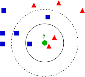
As shown above, there are two different types of sample data, each with a small blue square and small red triangle indicates that the middle of FIG green circle marked data is data to be classified. That, now, we do not know the middle of the green data is dependent on what kind of (small blue squares or small red triangle), KNN is to solve this problem.

If K = 3, the most recent three neighbors green dot is two small red triangle and a little blue square, minority subordinate to the majority, based on the statistical method of determining the classification to be green this point belongs to a red triangle class.

If K = 5, the most recent five neighbors green dot is two red triangles and three blue squares, a minority subordinate to the majority, based on the statistical method of determining the classification to be green this point belongs to the blue square one type.

Here we see that when the current to be unable to determine the classification point is subordinate to the known classification of what type, we can look at it based on the position of features in which the theory of statistics, measure it right around the neighbor's heavy, but the it is classified as (or assigned) to a greater weight of the kind. This is the core idea of K nearest neighbor algorithm.

1.2 nearest neighbor distance metric

We see that the core of K nearest neighbor algorithm is to find examples of neighbor points, this time, on the heels of the problem, how to find a neighbor, the neighbor is what criteria, what to measure. This series of questions is to talk about the measure from the following notation.

What distance metric notation (universal knowledge, you can skip):

Euclidean distance , the most common distances between two or more points notation, also known as the Euclidean metric, which is defined in Euclidean space, such as the point x = (x1, ... the distance between, xn) and y = (y1, ..., yn ) is:

\[d(x,y)=\sqrt{(x_1-y_1)^2+(x_2-y_2)^2+...+(x_n-y_n)^2}=\sqrt{\sum_{i=1}^{n}(x_i-y_i)^2}\]
- Two-dimensional plane between two points on a (x1, y1) and b (x2, y2) Euclidean distance:
  
  \[d_{12}=\sqrt{(x_1-x_2)^2+(y_1-y_2)^2}\]
- Two three-dimensional space a (x1, y1, z1) and Euclidean between b (x2, y2, z2) from:
  
  \[d_{12}=\sqrt{(x_1-x_2)^2+(y_1-y_2)^2+(z_1-z_2)^2}\]
- Two n-dimensional vector a (x11, x12, ..., x1n) and b (x21, x22, ..., x2n) the Euclidean distance between:
  
  \[d_{12}=\sqrt{\sum_{k=1}^{n}(x_{1k}-x_{2k})^2}\]
  
  It may be expressed by the form of vector operations:
  
  \[d_{12}=\sqrt{(a-b)(a-b)^T}\]
Manhattan distance , we can define a formal sense L1- Manhattan distance is the distance or city block distance, i.e. the sum of two points on the line segment projected from the rectangular coordinate system fixed to the Euclidean space formed by shaft generated. For example, on a plane, the Manhattan distance between the point coordinates (x1, y1) of the point P1 and the coordinate (x2, y2) and P2 is: \ (| x_1-x_2 | + | Y_1-Y_2 | \) , to be noted that, Manhattan distance dependence of the rotation of the coordinate system, rather than a translation or mapping coordinate system axis.

Popular terms, imagine you drive from one intersection to another intersection in Manhattan, the driving distance between two points is a straight line from it? Obviously not, unless you can pass through the building. The actual driving distance is the "Manhattan distance", namely the source of the name of the Manhattan distance, at the same time, also known as the Manhattan city block distance from (City Block distance).
- Two two-dimensional plane a (x1, y1) and between b (x2, y2) of Manhattan distance
  
  \[d_{12}=|x_1-x_2|+|y_1-y_2|\]
- Manhattan distance between two n-dimensional vector a (x11, x12, ..., x1n) and b (x21, x22, ..., x2n)
  
  \[d_{12}=\sum_{k=1}^{n}|x_{1k}-x_{2k}|\]
Chebyshev distance , if the two vectors or two points p, and q, respectively, Pi and Qi, which is then cut between the two coordinate Chebyshev distance ratio is defined as follows:

\[D_{Chebyshev}(p,q)=max_i(|p_i-q_i|)\]

This is also equal to or less extremum measure Lp: \ (\ lim_ {X \ to \ infty} (\ sum_. 1 = {I}} ^ {n-| P_i-Q_I | ^ K). 1 ^ {/} K \) , Thus Chebyshev distance metric L∞ also known.

Mathematical viewpoint, Chebyshev distance by the same norm (uniform norm) (or referred to as supremum norm) derived metric, also a super Convex Metric (injective metric space) is.

In plane geometry, if the two-point coordinate Cartesian coordinates of p and q is (x1, y1) and (x2, y2), the Chebyshev distance of:

\ [D_ {Chess} = max (| x_2-x_1 |, | y_2-y_1 |) \]

Played chess friends may know, the king take the step to move to any one adjacent eight squares in. Then the king went to the grid (x2, y2) from the grid (x1, y1) requires a minimum of how many steps? . You will find the minimum number of steps is always max (| x2-x1 |, | y2-y1 |) steps. There is a similar kind of distance measurement method called Chebyshev distance.
- Two two-dimensional plane a (x1, y1) between the cut and the b (x2, y2) Chebyshev distance:
  
  \[d_{12}=max(|x_2-x_1|,|y_2-y_1|)\]
- Two n-dimensional vector a (x11, x12, ..., x1n) between the cut and the b (x21, x22, ..., x2n) Chebyshev distance:
  
  \[d_{12}=max_i(|x_{1i}-x_{2i}|)\]
  
  Another form of this equation is equivalent
  
  \[d_{12}=lim_{k\to\infin}(\sum_{i=1}^{n}|x_{1i}-x_{2i}|^k)^{1/k}\]
Minkowski distance (Minkowski Distance), Minkowski distance not a distance, but rather defines a set distance.

Two n-dimensional variable a (x11, x12, ..., x1n) and b (x21, x22, ..., x2n) between the Minkowski distance is defined as:

\[d_{12}=\sqrt[p]{\sum_{k=1}^{n}|x_{1k}-x_{2k}|^p}\]

Wherein p is a variable parameter.
When p = 1, the Manhattan distance is
when p = 2, is the Euclidean distance
when p → ∞, the Chebyshev distance is
depending on variable parameters, Minkowski distance may represent the distance of a class.
Standardized Euclidean distance , an improved standardization program for the shortcomings of the Euclidean distance is simply the Euclidean distance and made. Thinking standard Euclidean distance: Since dimensional distribution of the component data is not the same, that the individual components are first "standardized" to mean equal variance. As for the mean and variance normalized to the number, to review the statistical point of knowledge.

Suppose mathematical expectation or mean of sample set of X (mean) is m, the standard deviation (standard deviation, variance square root) is s, then the X's "normalized variables" X * is expressed as: (Xm) / s, and normalized variables mathematical expectation 0 and variance 1.
That is, the standardization process (Standardization) sample set is described by a formula:

\[X^*=\frac{X-m}{s}\]

= Normalized value (normalization value before - mean component) / standard deviation component　　
through simple derivation can be obtained two n-dimensional vector a (x11, x12, ..., x1n) and b (x21, x22, ... standardization between x2n) Euclidean distance formula:

\[d_{12}=\sqrt{\sum_{k=1}^{n}(\frac{x_{1k}-x_{2k}}{s_k})^2}\]
Mahalanobis distance

There are M samples vectors X1 ~ Xm, referred to as a covariance matrix S, referred to as the mean vector μ, the sample vectors X where u is the Mahalanobis distance is expressed as:

\[D(X)=\sqrt{(X-u)^TS^{-1}(X_i-X_j)}\]
- If the covariance matrix is the identity matrix (independent and identically distributed among the various sample vectors), the formula has become, that is, the Euclidean distance:
  
  \[D(X_i,X_j)=\sqrt{(X_i-X_j)^T(X_i-X_j)}\]
- If the covariance matrix is a diagonal matrix, equation becomes normalized Euclidean distance.
Advantages and disadvantages of the Mahalanobis distance: dimensionless nothing to eliminate interference correlation between variables.
Bhattacharyya distance

In statistics, Bhattacharyya distance to measure the similarity of two discrete or continuous probability distribution. It is closely related to the measure of the amount of overlap between the two statistical sample or population Pap distance coefficient. Bhattacharyya Bhattacharyya distance and distance factor to the 1930s, was named in a statistician working UIS India A. Bhattacharya. Meanwhile, the Bhattacharyya coefficient can be used to determine the two samples that are relatively close, which is used in the class classification separability measurement.

For discrete probability distribution p and q are the same domain in X, which is defined as:

\[D_B(p,q)=-ln(BC(p,q))\]

among them:

\[BC(p,q)=\sum_{x\in_{}X}\sqrt{p(x)q(x)}\]

Is the Bhattacharyya coefficient.
Hamming distance

Hamming distance is defined between two strings s1 and s2 as long as a minimum number of times in which the need to make a further alternative becomes. For example, the Hamming distance between the character string "1111" and "1001" is 2. Applications: information encoding (in order to enhance fault tolerance, such that the minimum Hamming distance between encoded as large as possible).
Cosine

Geometry angle cosine vector used to measure the differences between two directions, the machine learning concept borrowed to measure the difference between the sample vectors.
- Vector A (x1, y1) in two dimensions and vector B (x2, y2) of the cosine formula:
  
  \[cos\theta=\frac{x_1x_2+y_1y_2}{\sqrt{x_1^2+y_1^2}\sqrt{x_2^2+y_2^2}}\]
- Two n-dimensional sample points a (x11, x12, ..., x1n) and b (x21, x22, ..., x2n) cosine of the angle:
  
  \[cos\theta=\frac{a*b}{|a||b|}\]
Cosine of the angle in the range of [-1,1]. The larger the angle the cosine of the angle between two vectors is smaller, the greater the smaller the angle the cosine of the angle between two vectors. When the two vectors coincide with the direction cosine of the angle takes the maximum value 1, when the direction of two opposite cosine vectors minimum value -1.
Jaccard similarity coefficient

Two sets A and B of intersection of elements A, B and the proportion of concentrated, called two sets Jaccard similarity coefficient, indicated by symbol J (A, B). Jaccard similarity coefficient is an indicator to measure the similarity of two sets.

\[J(A,B)=\frac{|A\cap_{}B|}{|A\cup_{}B|}\]

Jaccard similarity coefficient with the opposite concept Jaccard Distance:

\[J_{\delta}(A,B)=1-J(A,B)=\frac{|A\cup_{}B|-|A\cap_{}B|}{|A\cup_{}B|}\]
Pearson coefficient

In statistics, Pearson product-moment correlation coefficient is a measure of correlation (linear correlation) between the two variables X and Y, a value between -1 and 1. Typically the variable is determined by the following correlation strength ranges:

0.8-1.0 highly relevant
0.6-0.8 strong correlation
0.4-0.6 moderate correlation
0.2-0.4 weak correlation
0.0-0.2 extremely weak correlation or no correlation

Simply put, all kinds of "distance" scenarios simply summarized as,

Space: Euclidean distance,
Path: Manhattan distance, Chess King: Chebyshev distance,
More than three forms of unity: Minkowski distance,
Weighted: normalized Euclidean distance,
Exclusion and interdependent dimensions: Mahalanobis distance,
Vector Gap: cosine,
Coding differences: Hamming distance,
Set approximation: Jaccard coefficient is similar to the distance,
Related: correlation coefficient correlation distance.

1.3 K value selection

If selecting a smaller value of K is equivalent to a predicted small training examples in the field of "learning" will reduce the approximation error, or similar training examples only closer to the input instance will act on the prediction result the problem at the same time bring the "learning" the estimation error increases, in other words, reducing the K value means that the overall model is complicated, prone to over-fitting;
If you choose a larger value of K is equivalent to the prediction with a large field of training examples, it has the advantage to reduce the estimation error learning, but the drawback is the learning approximation error increases. At this time, the input instance distant (dissimilar) training examples will also predictor role of the prediction error occurred, and the K value increases means that the overall model is simple.
K = N, is completely worthless, because at this time no matter what the input instance is just a simple prediction it belongs to the most tired in training examples, the model is too simple, ignoring a lot of useful information on training instances.

In practice, the value of K generally takes a relatively small value, for example, using cross-validation (simply, the training set is made part of the sample, a portion of the test set do) to choose the optimal K values.

1.4 KNN nearest neighbor classification algorithm process

Calculating test sample and the training samples from each sample point (common distance metric with a Euclidean distance, Mahalanobis distance, etc.);
All the above distance values are sorted;
Is selected from the k samples before a minimum distance;
Vote according to label these k samples to obtain a final classification category;

2. KDD implementation: KD tree

Kd- tree is an abbreviation K-dimension tree is k-dimensional data points in the space (two-dimensional (x, y), D (x, y, z), k dimensions (x1, y, z ..)) a data structure divided, mainly used in multidimensional space search key data (such as: search range and nearest neighbor search). Essentially, Kd- tree is a balanced binary tree.

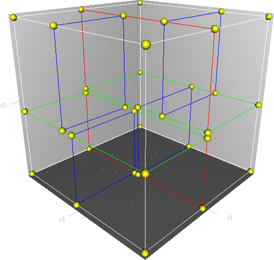
First of all it must be clear that, kd tree is a space partition tree, plainly, is to put the entire space is divided into specific sections, then search operation in the relevant part of a specific space. Imagine a three-dimensional (multidimensional little embarrassed your imagination) space, kd tree is divided according to certain rules of this three-dimensional space is divided into a plurality of spaces, as shown below:

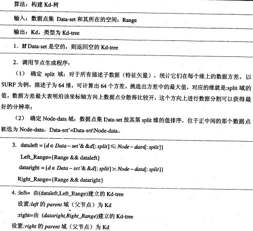
2.1 构建KD树

kd树构建的伪代码如下图所示：

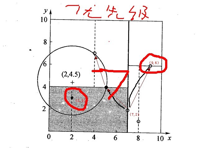
再举一个简单直观的实例来介绍k-d树构建算法。假设有6个二维数据点{(2,3)，(5,4)，(9,6)，(4,7)，(8,1)，(7,2)}，数据点位于二维空间内，如下图所示。为了能有效的找到最近邻，k-d树采用分而治之的思想，即将整个空间划分为几个小部分，首先，粗黑线将空间一分为二，然后在两个子空间中，细黑直线又将整个空间划分为四部分，最后虚黑直线将这四部分进一步划分。

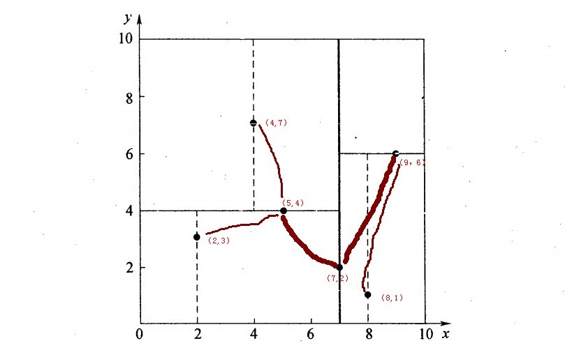
6个二维数据点{(2,3)，(5,4)，(9,6)，(4,7)，(8,1)，(7,2)}构建kd树的具体步骤为：

确定：split域=x。具体是：6个数据点在x，y维度上的数据方差分别为39，28.63，所以在x轴上方差更大，故split域值为x；
确定：Node-data = （7,2）。具体是：根据x维上的值将数据排序，6个数据的中值(所谓中值，即中间大小的值)为7，所以Node-data域位数据点（7,2）。这样，该节点的分割超平面就是通过（7,2）并垂直于：split=x轴的直线x=7；
确定：左子空间和右子空间。具体是：分割超平面x=7将整个空间分为两部分：x<=7的部分为左子空间，包含3个节点={(2,3),(5,4),(4,7)}；另一部分为右子空间，包含2个节点={(9,6)，(8,1)}；
如上算法所述，kd树的构建是一个递归过程，我们对左子空间和右子空间内的数据重复根节点的过程就可以得到一级子节点（5,4）和（9,6），同时将空间和数据集进一步细分，如此往复直到空间中只包含一个数据点。

与此同时，经过对上面所示的空间划分之后，我们可以看出，点(7,2)可以为根结点，从根结点出发的两条红粗斜线指向的(5,4)和(9,6)则为根结点的左右子结点，而(2,3)，(4,7)则为(5,4)的左右孩子(通过两条细红斜线相连)，最后，(8,1)为(9,6)的左孩子(通过细红斜线相连)。如此，便形成了下面这样一棵k-d树：

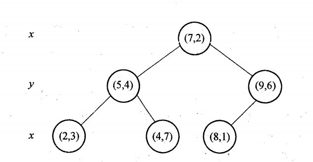
对于n个实例的k维数据来说，建立kd-tree的时间复杂度为O(knlogn)。

k-d树算法可以分为两大部分，除了上部分有关k-d树本身这种数据结构建立的算法，另一部分是在建立的k-d树上各种诸如插入，删除，查找(最邻近查找)等操作涉及的算法。下面，咱们依次来看kd树的插入、删除、查找操作。

2.2 KD树的插入

元素插入到一个K-D树的方法和二叉检索树类似。本质上，在偶数层比较x坐标值，而在奇数层比较y坐标值。当我们到达了树的底部，（也就是当一个空指针出现），我们也就找到了结点将要插入的位置。生成的K-D树的形状依赖于结点插入时的顺序。给定N个点，其中一个结点插入和检索的平均代价是O(log2N)。

插入的过程如下:

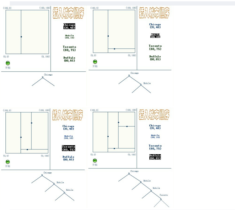
应该清楚，这里描述的插入过程中，每个结点将其所在的平面分割成两部分。因比，Chicago 将平面上所有结点分成两部分，一部分所有的结点x坐标值小于35，另一部分结点的x坐标值大于或等于35。同样Mobile将所有x坐标值大于35的结点以分成两部分，一部分结点的Y坐标值是小于10，另一部分结点的Y坐标值大于或等于10。后面的Toronto、Buffalo也按照一分为二的规则继续划分。

2.3 KD树的删除

KD树的删除可以用递归程序来实现。我们假设希望从K-D树中删除结点（a,b）。如果（a,b）的两个子树都为空，则用空树来代替（a,b）。否则，在（a,b）的子树中寻找一个合适的结点来代替它，譬如(c,d)，则递归地从K-D树中删除（c,d）。一旦(c,d)已经被删除，则用（c,d）代替（a,b）。假设(a,b)是一个X识别器，那么，它得替代节点要么是（a,b）左子树中的X坐标最大值的结点，要么是（a,b）右子树中x坐标最小值的结点。

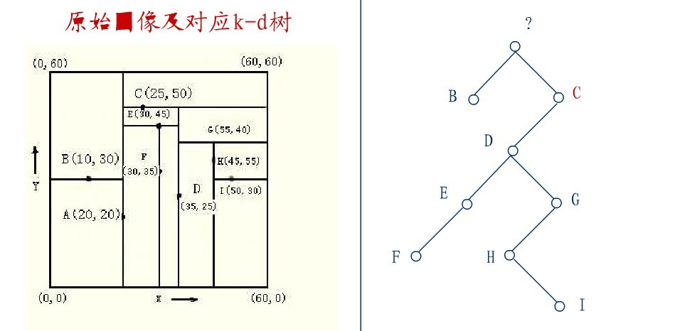
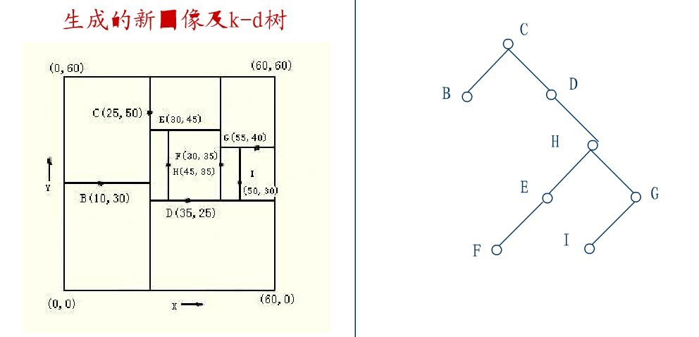
下面来举一个实际的例子(来源：中国地质大学电子课件，原课件错误已经在下文中订正)，如下图所示，原始图像及对应的kd树，现在要删除图中的A结点，请看一系列删除步骤：

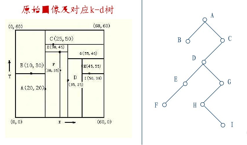
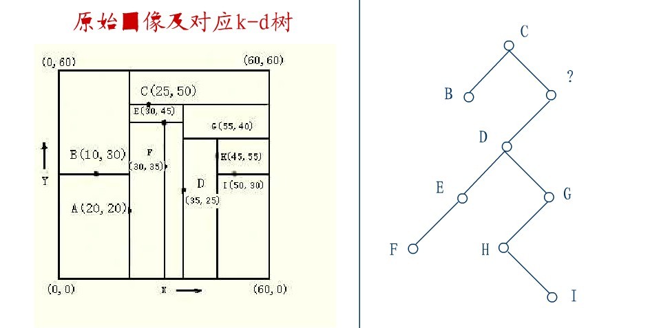
要删除上图中结点A，选择结点A的右子树中X坐标值最小的结点，这里是C，C成为根，如下图：

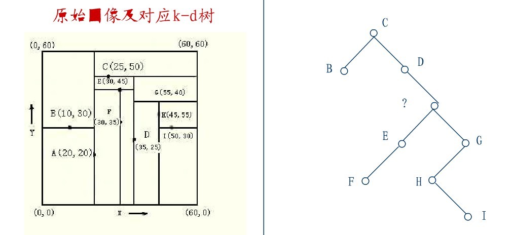
从C的右子树中找出一个结点代替先前C的位置，

这里是D，并将D的左子树转为它的右子树，D代替先前C的位置，如下图：

在D的新右子树中，找X坐标最小的结点，这里为H，H代替D的位置，

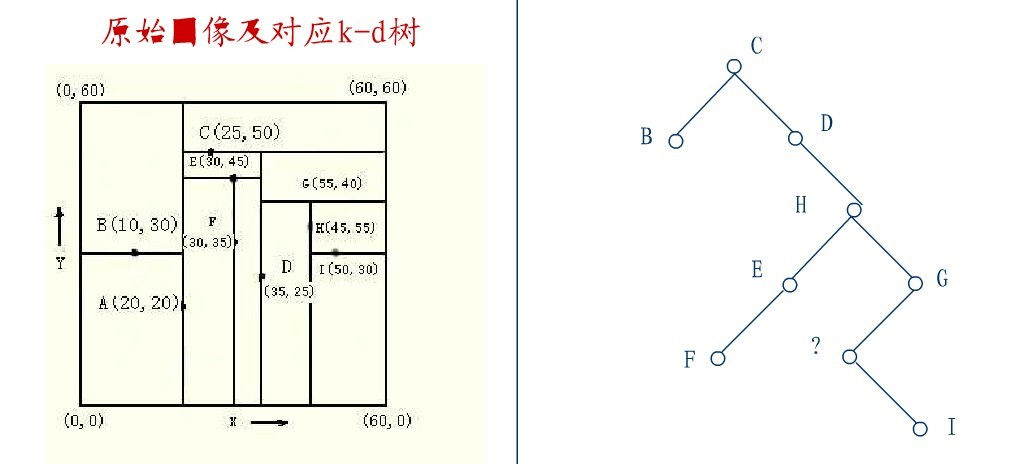
在D的右子树中找到一个Y坐标最小的值，这里是I，将I代替原先H的位置，从而A结点从图中顺利删除，如下图所示：

从K-D树中删除一个结点是代价很高的，很清楚删除子树的根受到子树中结点个数的限制。用TPL（T）表示树T总的路径长度。可看出树中子树大小的总和为TPL（T）+N。以随机方式插入N个点形成树的TPL是O(N*log2N),这就意味着从一个随机形成的K-D树中删除一个随机选取的结点平均代价的上界是O(log2N) 。

2.4 KD树的最近邻搜索算法

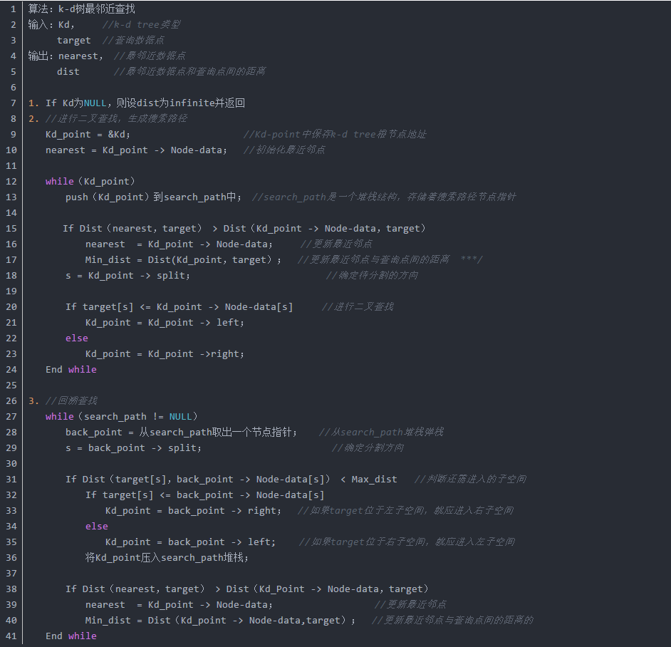
k-d树查询算法的伪代码如下所示：

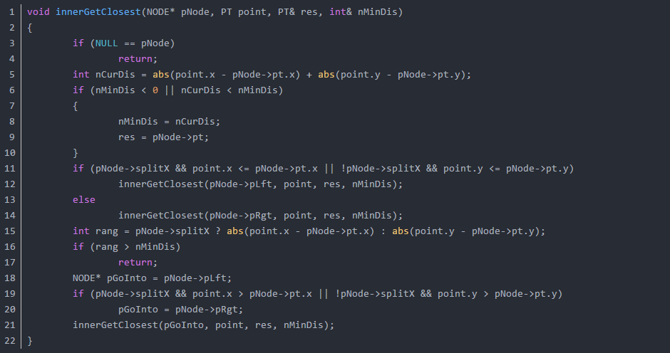
我写了一个递归版本的二维kd tree的搜索函数你对比的看看：

举例

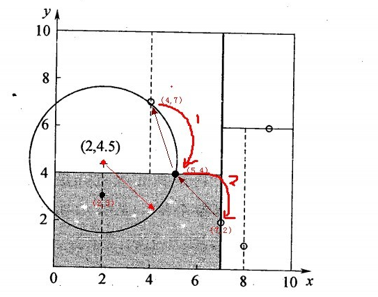
星号表示要查询的点查询点（2，4.5）。通过二叉搜索，顺着搜索路径很快就能找到最邻近的近似点。而找到的叶子节点并不一定就是最邻近的，最邻近肯定距离查询点更近，应该位于以查询点为圆心且通过叶子节点的圆域内。为了找到真正的最近邻，还需要进行相关的‘回溯'操作。也就是说，算法首先沿搜索路径反向查找是否有距离查询点更近的数据点。

二叉树搜索：先从（7,2）查找到（5,4）节点，在进行查找时是由y = 4为分割超平面的，由于查找点为y值为4.5，因此进入右子空间查找到（4,7），形成搜索路径<(7,2)，(5,4)，(4,7)>，但（4,7）与目标查找点的距离为3.202，而（5,4）与查找点之间的距离为3.041，所以（5,4）为查询点的最近点；
回溯查找：以（2，4.5）为圆心，以3.041为半径作圆，如下图所示。可见该圆和y = 4超平面交割，所以需要进入（5,4）左子空间进行查找，也就是将（2,3）节点加入搜索路径中得<(7,2)，(2,3)>；于是接着搜索至（2,3）叶子节点，（2,3）距离（2,4.5）比（5,4）要近，所以最近邻点更新为（2，3），最近距离更新为1.5；
回溯查找至（5,4），直到最后回溯到根结点（7,2）的时候，以（2,4.5）为圆心1.5为半径作圆，并不和x = 7分割超平面交割，如下图所示。至此，搜索路径回溯完，返回最近邻点（2,3），最近距离1.5。

2.5 kd树近邻搜索算法的改进：BBF算法

实例点是随机分布的，那么kd树搜索的平均计算复杂度是O（logN），这里的N是训练实例树。所以说，kd树更适用于训练实例数远大于空间维数时的k近邻搜索，当空间维数接近训练实例数时，它的效率会迅速下降，一降降到“解放前”：线性扫描的速度。

也正因为上述k最近邻搜索算法的第4个步骤中的所述：“回退到根结点时，搜索结束”，每个最近邻点的查询比较完成过程最终都要回退到根结点而结束，而导致了许多不必要回溯访问和比较到的结点，这些多余的损耗在高维度数据查找的时候，搜索效率将变得相当之地下，那有什么办法可以改进这个原始的kd树最近邻搜索算法呢？

从上述标准的kd树查询过程可以看出其搜索过程中的“回溯”是由“查询路径”决定的，并没有考虑查询路径上一些数据点本身的一些性质。一个简单的改进思路就是将“查询路径”上的结点进行排序，如按各自分割超平面（也称bin）与查询点的距离排序，也就是说，回溯检查总是从优先级最高（Best Bin）的树结点开始。

还是以上面的查询（2,4.5）为例，搜索的算法流程为：

将（7,2）压人优先队列中；
提取优先队列中的（7,2），由于（2,4.5）位于（7,2）分割超平面的左侧，所以检索其左子结点（5,4）。
同时，根据BBF机制”搜索左/右子树，就把对应这一层的兄弟结点即右/左结点存进队列”，将其（5,4）对应的兄弟结点即右子结点（9,6）压人优先队列中
此时优先队列为{（9,6）}，最佳点为（7,2）；然后一直检索到叶子结点（4,7），此时优先队列为{（2,3），（9,6）}，“最佳点”则为（5,4）；
提取优先级最高的结点（2,3），重复步骤2，直到优先队列为空。

2.6 KD树的应用

SIFT+KD_BBF搜索算法，详细参考文末的参考文献。

3. 关于KNN的一些问题

在k-means或kNN，我们是用欧氏距离来计算最近的邻居之间的距离。为什么不用曼哈顿距离？

答：我们不用曼哈顿距离，因为它只计算水平或垂直距离，有维度的限制。另一方面，欧式距离可用于任何空间的距离计算问题。因为，数据点可以存在于任何空间，欧氏距离是更可行的选择。例如：想象一下国际象棋棋盘，象或车所做的移动是由曼哈顿距离计算的，因为它们是在各自的水平和垂直方向的运动。
KD-Tree相比KNN来进行快速图像特征比对的好处在哪里?

答：极大的节约了时间成本．点线距离如果 >　最小点，无需回溯上一层，如果<,则再上一层寻找。