Convolutional neural network and the neural network is very similar to common: they have a learning weights and bias composed of neurons. Each neuron receives some input, performing the dot product, and optionally a nonlinear follow it.
The entire network can still exhibit a single differential Scoring:
One end of the pixel from the original image to the score of another class.
And on the last (fully connected) layer they still have a loss of function, and we are learning all the tricks of normal neural network development / still apply.
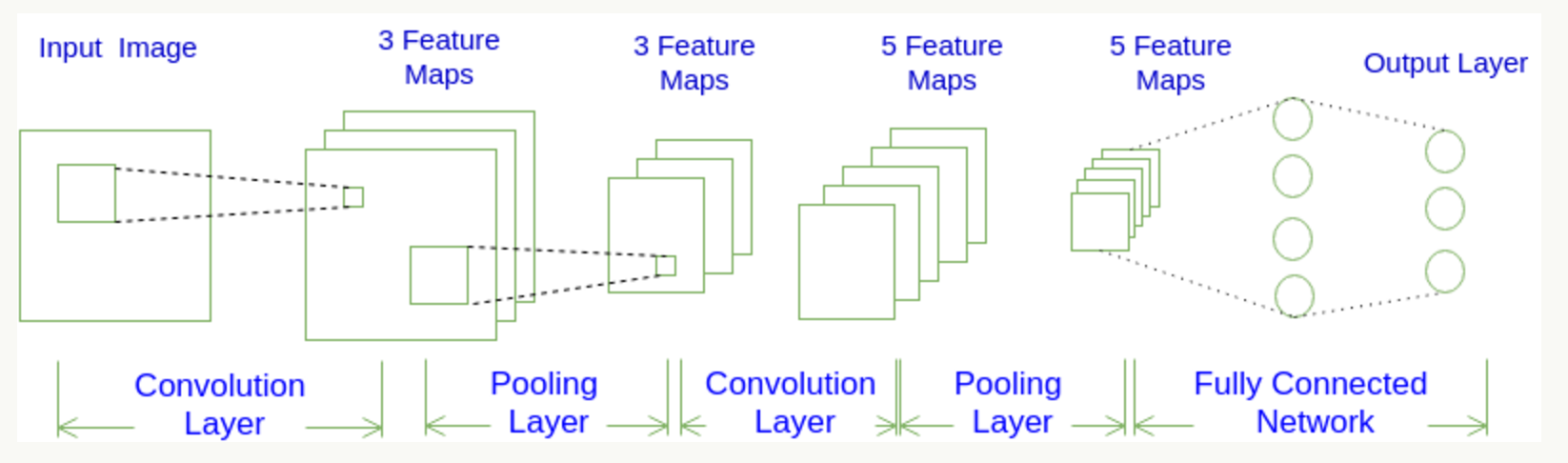
Each layer by CNN function differentiable an activation value into another, having a generally CNN convolution layer , cell layer and the fully connected layers the FC (as seen in the conventional neural network), the pool before there will be a general layer activation function, we will be stacking the layers to form a complete structure. We probably look at a map:

Convolution look at the development of neural networks:
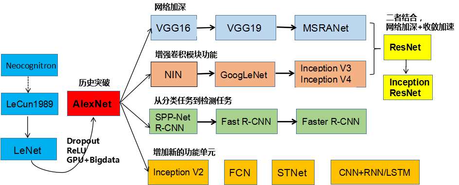

Error rate upgrade:


Convolution networking There are several kinds of architecture, name. The most common are:
-
LeNet. The first successful application of convolution network by Yann LeCun developed in the 1990s. One of the most famous is LeNet architecture for reading zip code, numbers and so on.
-
AlexNet. The network computer vision to promote the convolution first work is AlexNet, developed by Alex Kerry Wieruszewski, Ilya Sacijifu and Geoff Hinton. AlexNet be submitted to ImageNet ILSVRC challenge in 2012, significantly better than the second (compared to the runner-up, former five errors was 16%, 26% error). The network LeNet have very similar architecture, but a deeper, more and more features convolution stacked on top of each other (usually only one previous CONV tight layer with a layer POOL).
-
ZFNet。ILSVRC 2013获奖者是Matthew Zeiler和Rob Fergus的卷积网络。它被称为ZFNet(Zeiler&Fergus Net的缩写)。通过调整架构超参数,特别是通过扩展中间卷积层的大小,使第一层的步幅和过滤器尺寸更小,这是对AlexNet的改进。
-
GoogleNet。ILSVRC 2014获奖者是Szegedy等人的卷积网络。来自Google。其主要贡献是开发一个初始模块,大大减少了网络中的参数数量(4M,与AlexNet的60M相比)。此外,本文使用ConvNet顶部的“平均池”而不是“完全连接”层,从而消除了大量似乎并不重要的参数。GoogLeNet还有几个后续版本,最近的是Inception-v4。
-
VGGNet。2011年ILSVRC的亚军是来自Karen Simonyan和Andrew Zisserman的网络,被称为VGGNet。它的主要贡献在于表明网络的深度是良好性能的关键组成部分。他们最终的最佳网络包含16个CONV / FC层,并且吸引人的是,具有非常均匀的架构,从始至终只能执行3x3卷积和2x2池。他们预先训练的模型可用于Caffe的即插即用。VGGNet的缺点是评估和使用更多的内存和参数(140M)是更昂贵的。这些参数中的大多数都在第一个完全连接的层中,因此发现这些FC层可以在没有性能降级的情况下被去除,
-
ResNet。Kaiming He等人开发的残留网络 是ILSVRC 2015的获胜者。它具有特殊的跳过连接和批量归一化的大量使用。该架构在网络末端也缺少完全连接的层。读者也参考了凯明的演讲(视频,幻灯片),以及一些最近在火炬中复制这些网络的实验。ResNets目前是迄今为止最先进的卷积神经网络模型,并且是实际使用ConvNets的默认选择(截至2016年5月10日)。特别是,也看到最近从Kaiming He等人调整原有架构的发展。
然后介绍一下卷积神经网络的组件:
卷积层:
通过在原始图像上平移来提取特征,每一个特征就是一个特征映射:


就比如黄色的图片就是过滤器,我们利用它去卷积,过程如下:

外围补充与多Filter(P)
我们前面还曾提到,每个卷积层可以有多个filter。每个filter和原始图像进行卷积后,都可以得到一个Feature Map。因此,卷积后Feature Map的深度(个数)和卷积层的filter个数是相同的。
如果我们的步长移动与filter的大小不适合,导致不能正好移动到边缘怎么办?
这里就出现了零填充的大小P
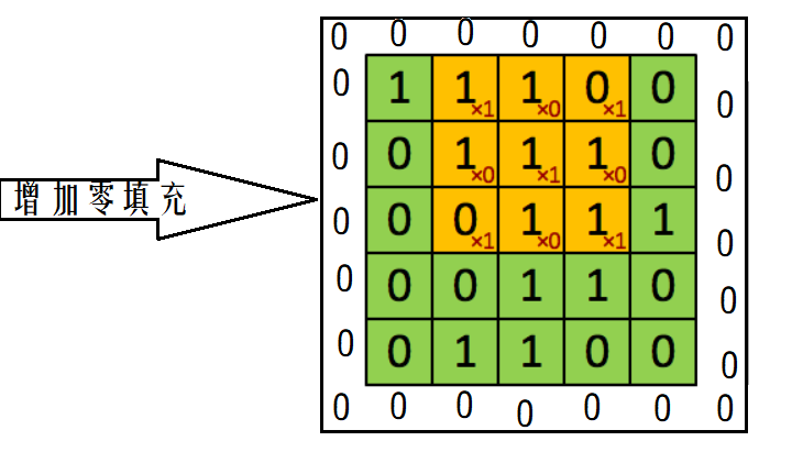

下图就是卷积层的计算方法。这里面体现了局部连接和权值共享:每层神经元只和上一层部分神经元相连(卷积计算规则),且filter的权值对于上一层所有神经元都是一样的。

卷积层过滤器:
-
个数 数量K :比如上图就是1个 大小 大小F: 比如上图就是filter:3*3 步长 步长S:比如上图就是1 零填充大小P
•卷积层输出深度、输出宽度
总结输出大小
-
输入体积大小H1∗W1∗D1
-
四个超参数:
-
Filter数量K
-
Filter大小F
-
步长S
-
零填充大小P
-
-
输出体积大小H2∗W2∗D2
-
H_2 = (H_1 - F + 2P)/S + 1
-
W_2 = (W_1 - F + 2P)/S + 1
-
D_2 = K
-
激活函数:
一般在进行卷积之后就会提供给激活函数得到一个输出值。我们不使用sigmoid,softmax,而使用Relu。该激活函数的定义是:
f(x)= max(0,x)
Relu函数如下:
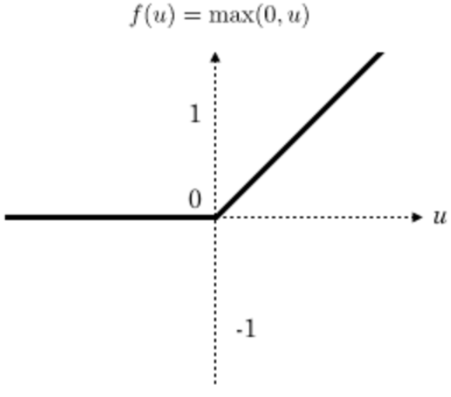
特点
-
速度快 和sigmoid函数需要计算指数和倒数相比,relu函数其实就是一个max(0,x),计算代价小很多
-
稀疏性 通过对大脑的研究发现,大脑在工作的时候只有大约5%的神经元是激活的,而采用sigmoid激活函数的人工神经网络,其激活率大约是50%。有论文声称人工神经网络在15%-30%的激活率时是比较理想的。因为relu函数在输入小于0时是完全不激活的,因此可以获得一个更低的激活率。
池化层:
通过特征后稀疏参数来减少学习的参数,降低网络的复杂度,(最大池化和平均池化)
Pooling层主要的作用是下采样,通过去掉Feature Map中不重要的样本,进一步减少参数数量。Pooling的方法很多,最常用的是Max Pooling。Max Pooling实际上就是在nn的样本中取最大值,作为采样后的样本值。


除了Max Pooing之外,常用的还有Mean Pooling——取各样本的平均值。对于深度为D的Feature Map,各层独立做Pooling,因此Pooling后的深度仍然为D。
全连接层:
那么在卷积网络当中,为什么需要加上FC层呢?
前面的卷积和池化相当于做特征工程,后面的全连接相当于做特征加权。最后的全连接层在整个卷积神经网络中起到“分类器”的作用
过拟合解决办法
Dropout(失活)
为了减少过拟合,我们在输出层之前加入dropout。我们用一个placeholder来代表一个神经元的输出在dropout中保持不变的概率。这样我们可以在训练过程中启用dropout,在测试过程中关闭dropout。 TensorFlow的tf.nn.dropout操作除了可以屏蔽神经元的输出外,还会自动处理神经元输出值的scale。所以用dropout的时候可以不用考虑scale。一般在全连接层之后进行Dropout
卷积神经网络的构建
一层卷积
卷积:32个filter,5*5,strides 1,padding="SAME"
输入:[None,28,28,1] 输出[None,28,28,32]
激活:[None,28,28,32]
池化:2*2,strides=2,padding="SAME"
输入:[None,28,28,32] 输出:[None,14,14,32]
偏置项:bias = 32
二层卷积
卷积:64个filter,5*5,strides=1,padding="SAME"
输入:[None,14,14,32] 输出[None,14,14,64]
激活:[None,14,14,64]
池化:2*2,strides=2,padding="SAME"
输入:[None,14,14,64] 输出:[None,7,7,64]
偏置项:bias = 64
全连接层FC:
输入:[None,7,7,64]-->[None,7*7*64]
权重:[None,7*7*64,10]
输出:[None,10]
偏置项:bias=10
import tensorflow as tf from tensorflow.examples.tutorials.mnist import input_data def weight_init(shape): w = tf.Variable(tf.random_normal(shape=shape,mean=0.0,stddev=1.0)) return w def bias_init(shape): b = tf.Variable(tf.constant(0.0,shape=shape)) return b def cnn(): # 1,初始化数据 mnist = input_data.read_data_sets("data/mnist/input_data/",one_hot=True) with tf.variable_scope("data"): x = tf.placeholder(tf.float32,[None,784]) y_true = tf.placeholder(tf.float32,[None,10]) # 2,第一层卷积 [None,784]-->[None,28,28,1] 5*5*1*32 strides=1-->[None,14,14,32] with tf.variable_scope("conv1"): x_reshape = tf.reshape(x,[-1,28,28,1]) w1 = weight_init([5,5,1,32]) b1 = bias_init([32]) # 卷积,激活,池化 x_relu1 = tf.nn.relu(tf.nn.conv2d(x_reshape,filter=w1,strides=[1,1,1,1],padding="SAME")+b1) x_poo11 =tf.nn.max_pool(x_relu1,ksize=[1,2,2,1],strides=[1,2,2,1],padding="SAME") # 3,第二层卷积 [None,14,14,32]--> 5*5*32*64 strides=1-->[None,7,7,64] with tf.variable_scope("conv2"): w2 = weight_init([5,5,32,64]) b2 = bias_init([64]) # 卷积,激活,池化 x_relu2 = tf.nn.relu(tf.nn.conv2d(x_poo11,filter=w2,strides=[1,1,1,1],padding="SAME")+b2) x_poo12 =tf.nn.max_pool(x_relu2,ksize=[1,2,2,1],strides=[1,2,2,1],padding="SAME") # 4,全连接层 [None,7,7,64]->[-1,7*7*64] w [7*7*64,10] b [10] with tf.variable_scope("full_connect"): w = weight_init([7*7*64,10]) b = bias_init([10]) x_fc_reshape = tf.reshape(x_poo12,shape=[-1,7*7*64]) y_predict = tf.matmul(x_fc_reshape,w)+b # 5,损失函数,梯度下降,模型评估 # 建立损失函数 with tf.variable_scope("soft_cross"): loss = tf.reduce_mean(tf.nn.softmax_cross_entropy_with_logits(labels=y_true, logits=y_predict)) # 梯度下降 with tf.variable_scope("optimizer"): train_op = tf.train.GradientDescentOptimizer(0.001).minimize(loss) # 模型评估 with tf.variable_scope("acc"): eq = tf.equal(tf.argmax(y_true, 1), tf.argmax(y_predict, 1)) accuracy = tf.reduce_mean(tf.cast(eq, tf.float32)) with tf.Session() as sess: tf.global_variables_initializer().run() for i in range(1000): x_mnist, y_mnist = mnist.train.next_batch(50) sess.run([train_op], feed_dict={x: x_mnist, y_true: y_mnist}) print("训练第%d步,准确率为:%f" % (i, sess.run(accuracy, feed_dict={x: x_mnist, y_true: y_mnist}))) return None if __name__ == '__main__': cnn()