table of Contents
2 matplotlib library to draw a histogram -hist ()
3 OpenCV library to draw a histogram -calcHist ()
Gray histogram Profile
1.1 histogram concept
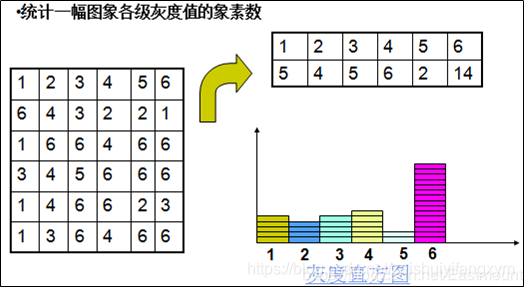
Histogram ( Histogram ) is the gray level function, described is the number of each gray level pixel image, reflecting an image of each frequency appear gray. Wherein the gray level is the abscissa, the ordinate is the frequency of occurrence of gray level.
1.2 histogram effect
1) When the contour line determination object boundary, the boundary threshold better choice by histogram thresholding process;
2) a strong contrast to the divided object and the background scenery is particularly useful;
3) Simple object area and the integrated optical density IOD can be determined by a histogram of the image.
1.3 Draw histogram
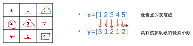
It assumed that there is a 3- 3 image, as shown in FIG array as
statistics is the gray level pixel array
count is the number of pixels having a gray level. Wherein the gradation pixels of 3 1, gradation of 1 pixel 2, pixel gray level of 2 to 3, the gradation of a total of 4 pixels, 5 pixels in total of gradation 2 a.
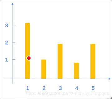
= [1, 2, 3, 4, 5]
= [3, 1, 2, 1, 2]
According to the above data, histograms plotted as follows:
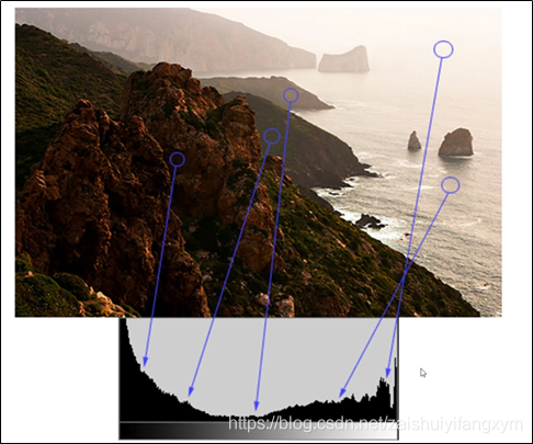
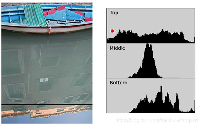
If the gray level 0-255 (minimum 0 black, 255 white a maximum value), corresponding to the same histogram can be drawn, the map is three and the mosaic image corresponding to the histogram.
1.4 normalized histogram
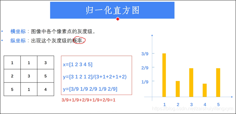
The histogram abscissa indicates the grayscale image, each pixel of ordinate represents the gradation occurrence probability . Calculated as follows:
The number (1) first calculates the gray level and the corresponding pixel
= [1, 2, 3, 4, 5]
= [3, 1, 2, 1, 2]
Number (2) total pixel count
= (3 + 1 + 2 + 1 +2) = 9
(3) 统计各个灰度级的出现概率
=
= [3/9, 1/9, 2/9, 1/9, 2/9]
2 matplotlib库 绘制直方图-hist()
使用matplotlib的子库pyplot实现,它提供了类似于Matlab的绘图框架,matplotlib是非常强大基础的一个Python绘图包。其中绘制直方图主要调用 hist() 函数实现,它根据数据源和像素级绘制直方图。
hist()函数形式如下:
hist(数据源, 像素级)
其中,参数:
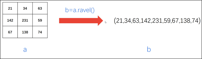
数据源:必须是一维数组,通常需要通过函数 ravel() 拉直图像
像素级:一般是256,表示[0, 255]
函数 ravel() 将多维数组降为一维数组,其格式为:
一维数组 = 多维数组.ravel()
代码如下所示:
#encoding:utf-8
import cv2
import numpy as np
import matplotlib.pyplot as plt
src = cv2.imread('zxp.jpg')
cv2.imshow("src", src)
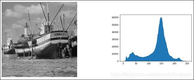
plt.hist(src.ravel(), 256)
plt.show()
cv2.waitKey(0)
cv2.destroyAllWindows()
运行结果如下图所示:
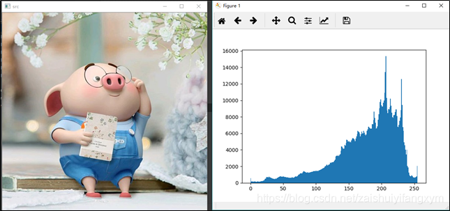
上述是调用 matplotlib库 中的hist() 函数来绘制直方图,接下来介绍使用OpenCV库中的calcHist() 函数绘制直方图。
3 OpenCV库 绘制直方图-calcHist()
使用OpenCV库中的 calcHist() 函数来绘制直方图:
hist = cv2.calcHist(images, channels, mask, histSize, ranges, accumulate)
Among them, the parameters:
hist histogram representing the return of a two-dimensional array;
images showing an original image;
channels represent the specified channel, the channel number in parentheses needed, when the input image is a grayscale image, it is [0], a color image was [0], [1], [2], B respectively, G, R;
mask histogram representing a mask image, the image of the entire statistical deputy, is set to None, when a certain part of the statistical histogram of the image, you need a mask image;
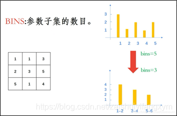
histSize BINS number representing the number, the subset of parameters, as shown below when the three bins = 3 represents a gray level;
ranges represents a pixel value range, such as [0, 255];
represents the cumulative accumulate overlay identifier defaults to false, if set to true, the histogram is not cleared at the start of dispensing, this parameter allows the calculation from the plurality of objects in a single histogram, or the histogram for real-time updates; accumulation result for a plurality of histograms of a set of image histogram calculation.
(1) calculating a basic size of the image gray scale, shape and content
Code as follows:
#encoding:utf-8
import cv2
import numpy as np
import matplotlib.pyplot as plt

src = cv2.imread('zxp.jpg')

# 参数:原图像 通道[0]-B 掩码 BINS为256 像素范围0-255
hist = cv2.calcHist([src], [0], None, [256], [0,255])
print('type=',type(hist))
print('size=',hist.size)
print('shape=',hist.shape)
print("-------------------")
print('hist=',hist)
Operating results as shown below:
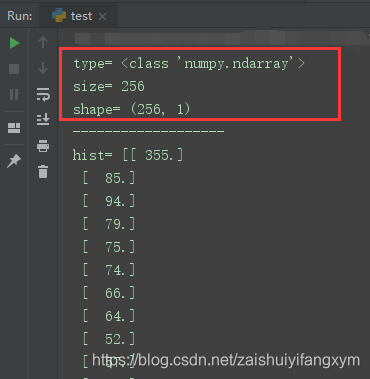
From the above results:
(1) is a histogram array;
(2) size of 256 ,;
(3) the shape of the line 256, one of an array.
(2) to add: matplotlib image rendering library
Code as follows:
#encoding:utf-8
import cv2
import numpy as np
import matplotlib.pyplot as plt
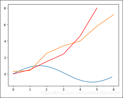
#绘制sin函数曲线
x1 = np.arange(0, 6, 0.1)
y1 = np.sin(x1)
plt.plot(x1, y1)
#绘制坐标点折现
x2 = [0, 1, 2, 3, 4, 5, 6]
y2 = [0.3, 0.4, 2.5, 3.4, 4, 5.8, 7.2]
plt.plot(x2, y2)
#省略有规则递增的x2参数
y3 = [0, 0.5, 1.5, 2.4, 4.6, 8]
plt.plot(y3, color="r")
plt.show()
Operating results as shown below:
(3) using OpenCV library calcHist () function to calculate B, G, R and gray level channel graphing
Code as follows:
#encoding:utf-8
import cv2
import numpy as np
import matplotlib.pyplot as plt

src = cv2.imread('zxp.jpg')

histb = cv2.calcHist([src], [0], None, [256], [0,255])
histg = cv2.calcHist([src], [1], None, [256], [0,255])
histr = cv2.calcHist([src], [2], None, [256], [0,255])

cv2.imshow("src", src)

plt.plot(histb, color='b')
plt.plot(histg, color='g')
plt.plot(histr, color='r')
plt.show()

cv2.waitKey(0)
cv2.destroyAllWindows()
Operating results as shown below:

Reference material
[1] https://blog.csdn.net/Eastmount/article/details/83758402