The tutorial uses matplotlib plotter command interface pyplot. The interface remains the global state, is useful for quickly and easily try a variety of graphics settings. Another approach is object-oriented interface, it is also very powerful, often more suitable for large-scale application development. If you want to learn object-oriented interface, then our usage guidelines are a good starting point.
First, start
Now, let us continue to use the command approach, first introduced into the relevant library
import matplotlib.pyplot as plt
import matplotlib.image as mpimg
Second, the image data into the array Numpy
Pillow library supports loading the image data. Matplotlib This machine only supports PNG images. If the unit fails to read, then the following command will return to the display Pillow.
The image used in this example is a JPG file, but remember that your "Pillow" requirements for their data.
This is the image we are dealing with:

Now we will load him into memory:
img = mpimg.imread('cat.jpg')
print(img)
[[[248 247 252]
  [248 247 252]
  [248 247 252]
  ...
  [253 252 255]
  [253 252 255]
  [253 252 255]]

 [[248 247 252]
  [248 247 252]
  [248 247 252]
  ...
  [253 252 255]
  [253 252 255]
  [253 252 255]]

 [[248 247 252]
  [248 247 252]
  [248 247 252]
  ...
Its output is a three-dimensional array. Each inner list represents a pixel. Here, the RGB image, there are three values. For RGBA image (wherein A is alpha or transparency), each having four internal list of values, but only simple image having a brightness value (therefore, it is only a 2-D array, instead of 3-D array). For RGB and RGBA image, matplotlib support float32 and uint8 data types. For gray, matplotlib only supports float32. If your array data does not meet one of the following description, you will need to re-adjust its size.
Third, the image will be drawn as numpy array
We can store data in numpy array (or generated by the introduction), then the image may be generated by rendering. In Matplotlib, this is the use of imshow () function to perform. Here, we will get drawing objects. This object provides you with an easy way to prompts from the graph.
import matplotlib.pyplot as plt
import matplotlib.image as mpimg

img = mpimg.imread('cat.jpg')

imgplot = plt.imshow(img)
plt.show()

The pseudo-color image is applied to the embodiment of FIG.
False color is a useful tool to more easily enhance contrast and visual data. When using the projector for presentations of data, which is especially useful - their generally poor contrast.
Only a single channel associated with pseudo-color, gradation, the luminance image. We currently have an RGB image (an array) (see the above content or data), we can choose a data channel:
lum_img = img[:, :, 0]
plt.imshow(lum_img)
plt.show()
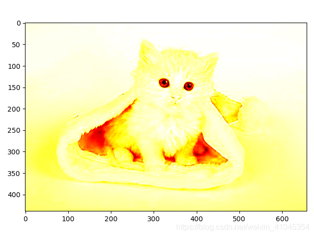
This time our cat looks a bit weird

Luminance (2D, no color) image, the color will be applied by default [FIG cmap] (also known as a look up table, LUT). The default name is viridis. There are many other options.
plt.imshow(lum_img, cmap="hot")
In addition, you can also use set_cmap () method to change the color map on an existing print objects, the role is consistent with the above, for example:
imgplot = plt.imshow(lum_img)
imgplot.set_cmap('nipy_spectral')
plt.show()
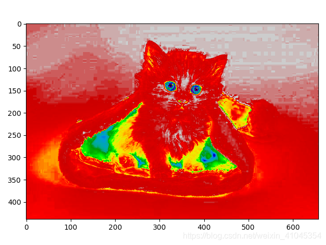
There are many other color map program. See color chart of the list and images
Color reference
Understanding color represents what the value would be helpful. We can do this by adding a color bar on your graphics:
imgplot = plt.imshow(lum_img)
imgplot.set_cmap('hot')
plt.colorbar()
plt.show()

Check specific data range
For a little bit of photography-based junior partner you should know histogram of the image. Sometimes you want to enhance the contrast of the image, or to expand specific areas of contrast, at the expense of color differences, small or insignificant these color changes. A histogram is a good tool to find interesting areas. To create the image data of the histogram , you can use hist () function.
plt.hist(img.ravel(), bins=256, range=(0.0, 255), fc='k', ec='k')

In most cases, the image of "interesting" portion is located around the peak, and may be obtained by an additional contrast and / or the lower region of the upper peak clipping. In our histogram, the end does not seem too useful information (image has a lot of white stuff). Let's adjust the upper limit, in order to effectively "amplify" part of the histogram. To this end, we will pass parameters to clim the imshow. You can also do this by calling set_clim () object image drawing method can also pass climparameters
imgplot = plt.imshow(lum_img, clim=(100, 255))

We compare the two figures together, the complete code:
import matplotlib.pyplot as plt
import matplotlib.image as mpimg

img = mpimg.imread('cat.jpg')
lum_img = img[:, :, 0]
fig1 = plt.figure()

plt.subplot(121)
plt.title('before')
imgplot = plt.imshow(lum_img)
plt.colorbar(orientation='horizontal')
plt.subplot(122)
plt.title('after')
imgplot2 = plt.imshow(lum_img, clim=(100, 255))
plt.colorbar(orientation='horizontal')
plt.show()
image:

Image interpolation (scaling)
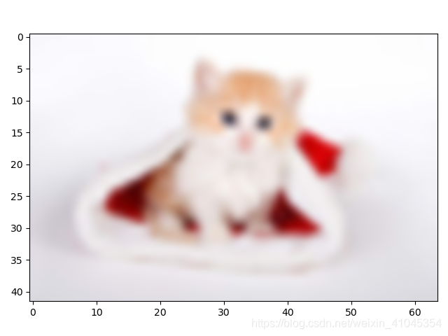
A common application is to adjust the image size, the number of pixels will change, so we need to calculate the increase (or delete) the value of the pixel based on different mathematical schemes. Because pixels are discrete and the lack of space. Interpolation is a way that you fill the space. This is why when you blow up the image sometimes may appear pixelated. When the bigger the difference between the original image and the expanded image, the effect will be more obvious. Let's narrow image. We are actually dropping pixels, leaving only a few pixels. Now, when we draw it, it will explode to the size of the data on the screen. The old pixel no longer exists, the computer must be extracted pixels to fill the space.
We will use Pillow library for loading images to resize the image.
from PIL import Image

img = Image.open('cat.jpg')
img.thumbnail((64, 64), Image.ANTIALIAS)  # resizes image in-place
imgplot = plt.imshow(img)
plt.show()

There is no default interpolation method, that is bilinear, because we did not give imshow () passing in any interpolation parameters.
We tried other methods. This is the "nearest", without interpolation.
imgplot = plt.imshow(img, interpolation="nearest")

It can be seen on the map and there is no difference, then try other parameters, often using bi-cubic interpolation is enlarged photograph - people tend to blur rather than pixelated:
imgplot = plt.imshow(img, interpolation="bicubic")