Computer Vision (Summary of Image Stitching Problems 1)

Preface

Because this "main line" of the computer vision course is over, I wrote this article to summarize the relevant knowledge of this important main line. I plan to divide this summary into 5 articles, which correspond to 5 steps.

text

First, let’s talk about several important steps of this main line in general. They are: "

The first step: feature point detection;

Step 2: Descriptor construction and adding descriptors;

Step 3: Match the feature points of the two images;

Step 4: Solve the linear transformation equations;

Step 5: Image Interpolation"

Next, I will give a detailed description of the knowledge points at each step, so please stay tuned!

1. Feature point detection

We want to select a feature point in an image, so what properties should this feature point have? Obviously, the feature point needs to have the following important properties:

1. Distinctiveness: Feature points should be unique in the image, that is, different image areas should have different feature points. This ensures that the corresponding feature points can be accurately found during the feature matching process.

2. Invariant: Feature points should have certain invariance to image rotation, scale changes, lighting changes, etc. This means that even under different image conditions, feature points in the same scene should be able to maintain similar descriptors for accurate matching.

3. Positioning accuracy (Localization): Feature points should be able to accurately locate their positions in the image. This is because the location information of feature points is an important input for subsequent processing tasks, so it requires high positioning accuracy.

4. Robustness: Feature points should have a certain degree of robustness against noise, occlusion, blur, etc. in the image. This means that the feature point detection algorithm should be able to extract accurate feature points under complex image conditions.

5. Repeatability: Feature points should appear repeatedly in different images. This is to ensure that the same feature points can be found in different images for cross-image matching and alignment.

So what algorithm should we use to select feature points? Here we will first talk about a method, which is the Harris corner point:

harris point

theory

Harris corner point is referred to as corner point. It actually does not fully satisfy the properties listed above, but let us forget about this first (). In short, we first think that there is such a corner point, which has the characteristics of stability, sparseness , special properties can be used as feature points of images. So, let us return to the core question, how to judge? My understanding here is to imagine a small window. If this small window moves very small in any direction, Distance can cause the pixel values ​​in it to change greatly, so this small window is the so-called corner point. So how do we describe this event from a mathematical perspective?

There is a set of quantitative evaluation rules for whether a point is a corner point. The evaluation index is: after the point area window (the size of the window is selected based on experience) is moved to a new position on the image, the pixels of the new window The difference between the value and the pixel value of the original window is 1. The window displacement at this time is deltaX and deltaY. The closer and smaller the deltaX and deltaY values ​​are, the more suitable the point is as a Harris corner point. In fact, the values ​​of deltaX and deltaY restrict each other. Their values ​​form an ellipse. We hope that this ellipse is a smaller perfect circle. After derivation, the size of the major and minor axes of the ellipse only depends on the pixels near the point in the image. information, and the pixel information near the position can be abstracted into ( Neighborhood window Second-order derivative matrix ): < /span>

This paragraph seems a bit difficult to understand. In my understanding, it means: "In Harris corner point detection, by calculating the eigenvalues ​​and determinants of the second-order derivative matrix, an elliptical shape can be obtained." If the major and minor axes of this ellipse are close and small, it means that the pixel distribution near the point has a large gradient change in both directions, and is therefore considered a corner point. Such an ellipse is usually considered to be approximately a perfect circle, indicating that the point is a stable corner point. The pixel information near the point can be abstracted into the second derivative matrix of the neighborhood window, which is the matrix "in the picture above"

Because of this, we can extract this expression from M to express how close the ellipse at this point is to a small-area perfect circle:

The K value here is still an empirical value, and when we use this expression, we need to determine whether the value of r(x) is greater than the threshold we set. If it is greater, then the x point is the corner point (Congratulations! !!)

So now that the mathematical principles are over, how do we use code to implement this corner detection? Next, let’s talk about the code part:

code

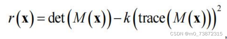
Let’s talk about the code part in words first. The code is divided into four steps. The first step is to find the first-order partial derivative for all pixels. The second step is to find the second-order partial derivative. The third step is to do a Gaussian blur. To sum up the second sister partial derivatives of all pixels in the domain window of each pixel, we actually want to get the M matrix. The fourth step is to use the r(x) formula above to find the value of each pixel. To determine whether it is a corner point, a simple code example is as follows:

import cv2
import numpy as np

# Step 1: 计算一阶偏导
def compute_gradients(image):
    dx = cv2.Sobel(image, cv2.CV_64F, 1, 0, ksize=3)  # 在x方向上计算一阶导数
    dy = cv2.Sobel(image, cv2.CV_64F, 0, 1, ksize=3)  # 在y方向上计算一阶导数
    return dx, dy

# Step 2: 计算二阶偏导
def compute_second_derivatives(dx, dy):
    Ixx = dx**2  # x方向上的二阶导数
    Ixy = dx * dy  # x和y方向上的混合导数
    Iyy = dy**2  # y方向上的二阶导数
    return Ixx, Ixy, Iyy

# Step 3: 计算M矩阵（通过高斯模糊）
def compute_m_matrix(Ixx, Ixy, Iyy, ksize):
    Ixx_blur = cv2.GaussianBlur(Ixx, (ksize, ksize), 0)  # 对Ixx进行高斯模糊
    Ixy_blur = cv2.GaussianBlur(Ixy, (ksize, ksize), 0)  # 对Ixy进行高斯模糊
    Iyy_blur = cv2.GaussianBlur(Iyy, (ksize, ksize), 0)  # 对Iyy进行高斯模糊
    return Ixx_blur, Ixy_blur, Iyy_blur

# Step 4: 计算角点响应函数值
def compute_harris_response(Ixx_blur, Ixy_blur, Iyy_blur, k=0.04):
    det_M = Ixx_blur * Iyy_blur - Ixy_blur**2  # M矩阵的行列式
    trace_M = Ixx_blur + Iyy_blur  # M矩阵的迹
    r = det_M - k * trace_M**2  # Harris角点响应函数
    return r

# 阈值化，得到角点
def detect_corners(image, threshold):
    dx, dy = compute_gradients(image)
    Ixx, Ixy, Iyy = compute_second_derivatives(dx, dy)
    ksize = 5  # 高斯模糊的核大小
    Ixx_blur, Ixy_blur, Iyy_blur = compute_m_matrix(Ixx, Ixy, Iyy, ksize)
    r = compute_harris_response(Ixx_blur, Ixy_blur, Iyy_blur)
    corners = np.where(r > threshold)  # 大于阈值的点被认为是角点
    return corners

# 读取图像
image = cv2.imread('image.jpg', 0)  # 读取灰度图像
threshold = 100000  # 阈值，用于筛选角点
corners = detect_corners(image, threshold)

# 在图像上绘制角点
for corner in zip(*corners):
    x, y = corner
    cv2.circle(image, (y, x), 5, 255, -1)  # 在角点位置画圆

# 显示结果
cv2.imshow('Corners', image)  # 显示包含角点的图像
cv2.waitKey(0)
cv2.destroyAllWindows()

By the way, let’s add some explanation of Gaussian blur here:

Gaussian blur is a commonly used image processing technique used to reduce noise and details in images to make them smoother. Its basic idea is to perform a weighted average of each pixel in the image according to the weight of its surrounding pixels, where the weight is determined by a Gaussian function.

The Gaussian function is a bell-shaped curve with the following properties:

1. **Maximum center:** The center of the curve has the maximum value, that is, the pixel itself has the highest weight.
2. **Symmetry:** The curve is symmetrical at the center point, ensuring smoothness.
3. **Graduality:** The values ​​on both sides of the curve gradually decrease, so pixels farther from the center point have lower weights.

In Gaussian blur, for each pixel in the image, the surrounding pixel values ​​are weighted and averaged according to the weight of the Gaussian function to obtain a new pixel value. This allows noise and detail in the image to be smoothed out, resulting in a blurrier image.

In image processing, Gaussian blur is often used in preprocessing to reduce image noise, or in some specific tasks, such as image smoothing before edge detection. The degree of Gaussian blur (that is, the degree of blur) is controlled by a parameter σ (sigma). The larger the σ value, the higher the degree of blur.

In actual image processing libraries (such as OpenCV), you can use built-in functions to perform Gaussian blur operations. These functions automatically calculate weights and perform weighted averaging without manual implementation of the Gaussian function.

SIFT feature points

theory

Since the Harris corner points we saw above actually have various problems, such as being invariant to illumination changes other than overall illumination changes, and not being deformable to geometric transformations other than rotation and translation transformations. So we A descriptor that satisfies scale invariance and rotation invariance was selected, which is the SIFT feature point extraction algorithm.

SIFT (Scale-Invariant Feature Transform) is a feature extraction algorithm used in image processing and computer vision. It has scale invariance (Scale Invariance) and rotation invariance (Rotation Invariance), which means that it can Stably detect and describe feature points in images under rotation angles. The following is a detailed introduction to the underlying principles of SIFT feature point extraction:

1. Scale Space Extrema Detection

SIFT first detects extreme points in the image by constructing a scale space. These extreme points exist stably at different scales. To achieve scale invariance, SIFT uses Gaussian filters to smooth images at different scales. At each scale, a series of images (Gaussian pyramids) are obtained by convolving the images with Gaussian kernel functions of different scales, and then looking for local extreme points on the images at each scale. These extreme points may be key point.

2. Key Point Localization

Based on the scale space extreme points, SIFT accurately locates the detected extreme points and determines the location of key points with sub-pixel level accuracy. SIFT uses neighboring pixels in scale space for fitting to find the sub-pixel positions of key points, which can improve the accuracy of key points.

3. Assigning Orientations to Key Points

To maintain rotation invariance, SIFT assigns a main direction to each keypoint. SIFT calculates the gradient magnitude and direction in the image area around the key point, then constructs a gradient histogram, and selects the largest peak in the histogram as the main direction of the key point. This ensures that feature points of the same scene have the same description at different angles.

In general, SIFT extracts feature points with scale invariance and rotation invariance in the image by constructing scale space, key point positioning, direction assignment and key point description. These feature points can be used for many computer vision tasks, such as object recognition, image stitching, etc.

The teacher here is not very detailed...

code

import cv2

# 读取图像
image = cv2.imread('image.jpg')
gray_image = cv2.cvtColor(image, cv2.COLOR_BGR2GRAY)

# 创建SIFT对象
sift = cv2.SIFT_create()

# 检测关键点
keypoints, descriptors = sift.detectAndCompute(gray_image, None)

# 在图像上绘制关键点
output_image = cv2.drawKeypoints(gray_image, keypoints, image)

# 显示结果
cv2.imshow('SIFT Keypoints', output_image)
cv2.waitKey(0)
cv2.destroyAllWindows()

Yes, I called this function directly, hahaha

Conclusion to part one

In short, the feature point detection part is over here!!