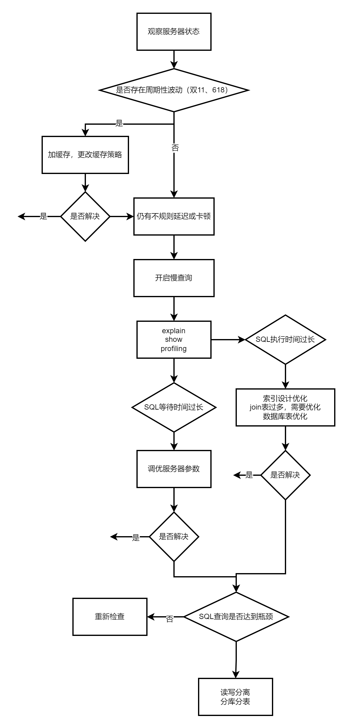
数据库性能分析工具的使用
在数据库调优中,我们的目标就是相应时间更快,吞吐量更大。利用宏观监控工具和微观日志分析可以帮我们快速找到调优的思路和方式。
1. 数据库服务器优化步骤
2. 查看系统性能参数
在MySQL种,可以使用show status 语句查询一些MySQL数据库服务器的性能参数和执行频率。
在MySQL中,可以使用 SHOW STATUS 语句查询一些MySQL数据库服务器的性能参数、执行频率。
SHOW STATUS语句语法如下:
SHOW [GLOBAL|SESSION] STATUS LIKE '参数';
一些常用的性能参数如下:
- Connections:连接MySQL服务器的次数。
- Uptime:MySQL服务器的上线时间。
- Slow_queries:慢查询的次数。
- Innodb_rows_read:Select查询返回的行数
- Innodb_rows_inserted:执行INSERT操作插入的行数
- Innodb_rows_updated:执行UPDATE操作更新的 行数
- Innodb_rows_deleted:执行DELETE操作删除的行数
- Com_select:查询操作的次数。
- Com_insert:插入操作的次数。对于批量插入的 INSERT 操作,只累加一次。
- Com_update:更新操作 的次数。
- Com_delete:删除操作的次数。
3. 统计SQL的查询成本:last_query_cost
一条SQL查询语句在执行前需要查询执行计划,如果存在多种执行计划的话,MySQL会计算每个执行计划所需要的成本,从中选择成本最小的一个作为最终执行的执行计划。
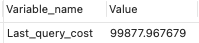
如果我们想要查看某条SQL语句的查询成本,可以在执行完这条SQL语句之后,通过查看当前会话中的last_query_cost变量值来得到当前查询的成本。它通常也是我们评价一个查询的执行效率的一个常用指标。这个查询成本对应的是SQL 语句所需要读取的读页的数量。
# 在命令行或使用navicat同时执行生效,用datagrip工具不生效
SELECT student_id, class_id, NAME, create_time
FROM student_info
WHERE id < 900001;

SHOW STATUS LIKE 'last_query_cost';
4. 定位执行慢的SQL:慢查询日志
MySQL的慢查询日志,用来记录在MysQL中响应时间超过阀值的语句,具体指运行时间超过long_query_time值的SQL,则会被记录到慢查询日志中。long_query_time的默认值为10,意思是运行10秒以上(不含10秒)的语句,认为是超出了我们的最大忍耐时间值。
它的主要作用是,帮助我们发现那些执行时间特别长的sQL查询,并且有针对性地进行优化,从而提高系统的整体效率。当我们的数据库服务器发生阻塞、运行变慢的时候,检查一下慢查询日志,找到那些慢查询,对解决问题很有帮助。比如一条sql执行超过5秒钟,我们就算慢SQL,希望能收集超过5秒的sql,结合explain进行全面分析。
默认情况下,MySQL数据库没有开启慢查询日志,需要我们手动来设置这个参数。如果不是调优需要的话,一般不建议启动该参数,因为开启慢查询由志会或多或少带来一定的性能影响。
慢查询日志支持将日志记录写入文件。
4.1 开启慢查询日志
(临时方式)
4.1.1 开启slow_query_log
# 查看变量值 默认OFF
show variables like '%slow_query_log%';
# 设置为on
set global slow_query_log = on;
# 设置之后可以看到查询出现了日志文件../mysql/data/localhost-slow.log
4.1.2 修改long_query_time阈值
show variables like '%long_query_time%';
# 全局和当前session变量修改
set global long_query_time = 1;
set long_query_time = 1;
补充:学习过MySQL变量可知,上面的操作只是对本次MySQL服务器有效,若服务器重启,则会失效。若想永久有效,需要修改MySQL的配置文件my.cnf
(永久方式)
[mysqld]
slow_query_log=ON   #开启慢查询日志的开关slow_query_log_file=/var/lib/mysql/localhost-slow.log  #慢查询日志的目录和文件名信息
long_query_time=3   #设置慢查询的阙值为3秒,超出此设定值的SQL即被记录到慢查询日志
log_output=FILE
4.1.3 案例演示
# 慢sql(execution: 1 s 82 ms, fetching: 14 ms)
SELECT s.name
FROM student_info s
         JOIN course c on s.course_id = c.course_id
GROUP BY s.name

# 查看慢查询日志数量
SHOW GLOBAL STATUS LIKE '%Slow_queries%'
4.1.4 慢查询日志分析工具:mysqldumpslow
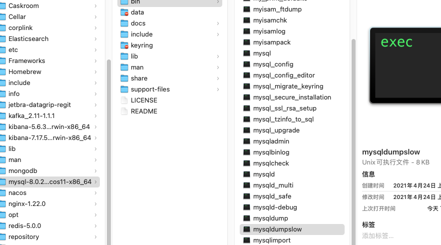
终端执行,注意这里不是在myslq里执行了,而是要用这个工具;
查看用法:
cat bin % ./mysqldumpslow -help
Usage: mysqldumpslow [ OPTS... ] [ LOGS... ]

Parse and summarize the MySQL slow query log. Options are

  --verbose    verbose
  --debug      debug
  --help       write this text to standard output

  -v           verbose
  -d           debug
  -s ORDER     what to sort by (al, at, ar, c, l, r, t), 'at' is default
                al: average lock time
                ar: average rows sent
                at: average query time
                 c: count
                 l: lock time
                 r: rows sent
                 t: query time
  -r           reverse the sort order (largest last instead of first)
  -t NUM       just show the top n queries
  -a           don't abstract all numbers to N and strings to 'S'
  -n NUM       abstract numbers with at least n digits within names
  -g PATTERN   grep: only consider stmts that include this string
  -h HOSTNAME  hostname of db server for *-slow.log filename (can be wildcard),
               default is '*', i.e. match all
  -i NAME      name of server instance (if using mysql.server startup script)
  -l           don't subtract lock time from total time
查看慢sql日志:
cat bin % ./mysqldumpslow -s t -t 5 /usr/local/mysql/data/localhost-slow.log

Reading mysql slow query log from /usr/local/mysql/data/localhost-slow.log
Count: 2  Time=1.07s (2s)  Lock=0.00s (0s)  Rows=501.0 (1002), root[root]@localhost
  /* ApplicationName=DataGrip N.N.N */ SELECT s.name
  FROM student_info s
  JOIN course c on s.course_id = c.course_id
  GROUP BY s.name

Died at ./mysqldumpslow line 162, <> chunk 2.
cat bin %
5. 查看SQL执行成本show profile(将弃用)
# 在命令行或使用navicat同时执行生效,用datagrip工具不生效
SELECT s.name
FROM student_info s
JOIN course c on s.course_id = c.course_id
GROUP BY s.name;
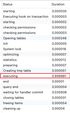
show profile;
可以看到是执行时间比较慢:
show profile的常用查询参数:
① ALL:显示所有的开销信息。
② BLOCK IO:显示块IO开销。
③ CONTEXT SWITCHES:上下文切换开销。
④ CPU:显示CPU开销信息。
⑤ IPC:显示发送和接收开销信息。
⑥ MEMORY:显示内存开销信 息。
⑦ PAGE FAULTS:显示页面错误开销信息。
⑧ SOURCE:显示和Source_function,Source_file, Source_line相关的开销信息。
⑨ SWAPS:显示交换次数开销信息。
日常开发需注意的结论:
① converting HEAP to MyISAM: 查询结果太大,内存不够,数据往磁盘上搬了。
② Creating tmp table:创建临时表。先拷贝数据到临时表,用完后再删除临时表。
③ Copying to tmp table on disk:把内存中临时表复制到磁盘上,警惕!
④ locked。
如果在show profile诊断结果中出现了以上4条结果中的任何一条,则sql语句需要优化。
注意:
不过SHOW PROFILE命令将被启用,我们可以从 information_schema 中的 profiling 数据表进行查看。
6. 分析查询语句:EXPLAIN
6.1 概述
定位了查询慢的 SQL之后,我们就可以使用 EXPLAIN 或 DESCRIBE 工具做针对性的分析查询语句。DESCRIBE语句的使用方法与EXPLAIN语句是一样的,并且分析结果也是一样的。
MySQL中有专门负责优化SELECT语句的优化器模块,主要功能: 通过计算分析系统中收集到的统计信息,为客户端请求的Query提供它认为最优的 执行计划 (他认为最优的数据索方式,但不见得是DBA认为是最优的,这部分最耗费时间)。
这个执行计划展示了接下来具体执行查询的方式,比如多表连接的顺序是什么,对于每个表采用什么访问方法来具体执行查询等等。MySQL为我们提供了 EXPLAIN语句来帮助我们查看某个查询语句的具体执行计划,大家看懂EXPLAIN语句的各个输出项,可以有针对性的提升我们查询语句的性能。
1. 能做什么?
- 表的读取顺序
- 数据读取操作的操作类型
- 哪些索引可以使用
- 哪些索引被实际使用
- 表之间的引用
- 每张表有多少行被优化器查询
2. 官网介绍
https://dev.mysql.com/doc/refman/5.7/en/explain-output.html
https://dev.mysql.com/doc/refman/8.0/en/explain-output.html
3. 版本情况
- MySQL 5.6.3以前只能 EXPLAIN SELECT ;MYSQL 5.6.3以后就可以 EXPLAIN SELECT,UPDATE, DELETE
- 在5.7以前的版本中,想要显示 partitions 需要使用 explain partitions 命令;想要显示 filtered 需要使用 explain extended 命令。在5.7版本后,默认explain直接显示partitions和 filtered中的信息。
6.2 基本语法
EXPLAIN 或 DESCRIBE语句的语法形式如下:
EXPLAIN SELECT select_options
或者
DESCRIBE SELECT select_options
If we want to see the execution plan of a certain query, we can add an EXPLAIN in front of the specific query statement, like this:
mysql> EXPLAIN SELECT 1;
EXPLAIN SELECT * FROM student_info;
| id | select_type | table | partitions | type | possible_keys | key | key_len | ref | rows | filtered | Extra |
|---|---|---|---|---|---|---|---|---|---|---|---|
| 1 | DELETE | student_info | NULL | range | PRIMARY | PRIMARY | 4 | const | 1 | 100 | Using where |
EXPLAINThe statement is used to analyze the execution plan of a MySQL query. It can help developers and DBAs understand how the query is optimized and executed, so as to optimize and adjust the query. EXPLAINThe functions of each column output by the statement are as follows:
-
id: Indicates the identifier of the operation in the query. For complex queries, there will be multiple operation steps. The id indicates the order of execution steps. The larger the id, the closer the execution order. back.
-
select_type: Indicates the type of query, which mainly includes the following types:
- SIMPLE: Simple query, does not contain subqueries or UNION.
- PRIMARY: The outermost query.
- SUBQUERY: A subquery that is part of another query.
- DERIVED: A query that derives a table, such as a subquery in the FROM clause.
-
table: Indicates the name of the table being accessed.
-
partitions: Indicates matching partitions if the table uses partitioning technology.
-
type: Indicates the access type of the table and is an important indicator of performance evaluation. Common types are:
- const: indicates that matching rows are found through the index once, usually used for primary key or unique index queries.
- ref: indicates using a non-unique index to find matching rows, usually used for queries using non-unique indexes or unique indexes.
- range: Indicates using the index range to find matching rows, usually used for using range queries on index columns.
- index: indicates a full table scan, traversing the entire index tree.
- all: indicates a full table scan, traversing the entire data table.
-
possible_keys: Indicates indexes that may be used in the query.
-
key: Indicates the actual index used.
-
key_len: Indicates the length of the actually used index, in bytes.
-
ref: Indicates how the index field used in the query is compared with the index.
-
rows: Indicates the estimated number of rows that need to be scanned.
-
filtered: Indicates the percentage of rows that are filtered out based on the conditions on the table.
-
Extra: Indicates additional information. Some common additional information are:
- Using index: Indicates that the query uses a covering index and does not need to access the original data of the table.
- Using where: indicates that filtering needs to be done on the MySQL server, not in the storage engine.
- Using temporary: Indicates that the query uses a temporary table to process the result set.
- Using filesort: Indicates that the query requires file sorting of the results.
By understanding each column output by the EXPLAIN statement, you can better understand the query execution plan, so as to perform performance optimization and index design.
6.3 Data preparation
CREATE TABLE s1
(
    id           INT AUTO_INCREMENT,
    key1         VARCHAR(100),
    key2         INT,
    key3         VARCHAR(100),
    key_part1    VARCHAR(100),
    key_part2    VARCHAR(100),
    key_part3    VARCHAR(100),
    common_field VARCHAR(100),
    PRIMARY KEY (id),
    INDEX idx_key1 (key1),
    UNIQUE INDEX idx_key2 (key2),
    INDEX idx_key3 (key3),
    INDEX idx_key_part (key_part1, key_part2, key_part3)
) ENGINE = INNODB
  CHARSET = utf8;

CREATE TABLE s2
(
    id           INT AUTO_INCREMENT,
    key1         VARCHAR(100),
    key2         INT,
    key3         VARCHAR(100),
    key_part1    VARCHAR(100),
    key_part2    VARCHAR(100),
    key_part3    VARCHAR(100),
    common_field VARCHAR(100),
    PRIMARY KEY (id),
    INDEX idx_key1 (key1),
    UNIQUE INDEX idx_key2 (key2),
    INDEX idx_key3 (key3),
    INDEX idx_key_part (key_part1, key_part2, key_part3)
) ENGINE = INNODB
  CHARSET = utf8;

# 创建函数,假如报错,需开启如下命令:允许创建函数设置:
# 不加global只是当前窗口有效。
set global log_bin_trust_function_creators = 1;

#该函数会返回一个字符串
DELIMITER //
CREATE FUNCTION rand_string1(n INT) RETURNS VARCHAR(255)
BEGIN
    DECLARE chars_str VARCHAR(100) DEFAULT 'abcdefghijklmnopqrstuvwxyzABCDEFJHIJKLMNOPQRSTUVWXYZ';
    DECLARE return_str VARCHAR(255) DEFAULT '';
    DECLARE i INT DEFAULT 0;
    WHILE i < n
        DO
            SET return_str = CONCAT(return_str, SUBSTRING(chars_str, FLOOR(1 + RAND() * 52), 1));
            SET i = i + 1;
        END WHILE;
    RETURN return_str;
END //
DELIMITER ;

# 创建往s1表中插入数据的存储过程:
DELIMITER //
CREATE PROCEDURE insert_s1(IN min_num INT(10), IN max_num INT(10))
BEGIN
    DECLARE i INT DEFAULT 0;SET autocommit = 0;
    REPEAT
        SET i = i + 1;
        INSERT INTO s1
        VALUES ((min_num + i), rand_string1(6), (min_num + 30 * i + 5), rand_string1(6), rand_string1(10), rand_string1(5), rand_string1(10),
                rand_string1(10));
    UNTIL i = max_num END REPEAT;
    COMMIT;
END //
DELIMITER ;

#创建往s2表中插入数据的存储过程:
DELIMITER //
CREATE PROCEDURE insert_s2(IN min_num INT(10), IN max_num INT(10))
BEGIN
    DECLARE i INT DEFAULT 0;SET autocommit = 0;
    REPEAT
        SET i = i + 1;
        INSERT INTO s2
        VALUES ((min_num + i), rand_string1(6), (min_num + 30 * i + 5), rand_string1(6), rand_string1(10), rand_string1(5), rand_string1(10),
                rand_string1(10));
    UNTIL i = max_num END REPEAT;
    COMMIT;
END //
DELIMITER ;

# 调用存储过程
# s1表数据的添加:加入1万条记录:
CALL insert_s1(10001, 10000);
# s2表数据的添加:加入1万条记录:
CALL insert_s2(10001, 10000);
6.4 The functions of each EXPLAIN column
In order to give everyone a better experience, we have adjusted the order of the output columns EXPLAIN.
1. table
No matter how complex our query statement is or how many tables it contains, in the end each table will need to be accessed by a single table. Therefore, MySQL stipulates that each record output by the EXPLAIN statement corresponds to a single table access. Method, the table column of the record represents the table name of the table (sometimes not the real table name, it may be the abbreviation).
EXPLAIN SELECT * FROM s1;

This query statement only involves a single-table query on the s1 table, so EXPLAIN There is only one record in the output, and the value of the table column is s1, indicating that this record is used Describes the single table access method to the s1 table.
Next we look at the execution plan of a join query
EXPLAIN SELECT * FROM s1 INNER JOIN s2;
| id | select_type | table | partitions | type | possible_keys | key | key_len | ref | rows | filtered | Extra |
|---|---|---|---|---|---|---|---|---|---|---|---|
| 1 | SIMPLE | s1 | null | ALL | null | null | null | null | 9895 | 100 | null |
| 1 | SIMPLE | s2 | null | ALL | null | null | null | null | 9895 | 100 | Using join buffer (hash join) |
It can be seen that there are two records in the execution plan of this connection query. The table columns of these two records are s1 and s2 respectively. These two records are used to describe the access methods to the s1 table and the s2 table respectively.
2. id
The query statements we write generally start with the SELECT keyword. A relatively simple query statement has only one SELECT keyword, such as the following query statement:
SELECT * FROM s1 WHERE key1 = 'a';
There is only one SELECT keyword in a slightly more complex connection query, such as:
SELECT * FROM s1 INNER JOIN s2
ON s1.key1 = s2.key1
WHERE s1.common_field = 'a';
For join queries, the FROM clause after a SELECT keyword can follow multiple tables, so in the execution plan of the join query, each table will correspond to a record, but the id values of these records are the same, for example :
EXPLAIN SELECT * FROM s1 INNER JOIN s2;
| id | select_type | table | partitions | type | possible_keys | key | key_len | ref | rows | filtered | Extra |
|---|---|---|---|---|---|---|---|---|---|---|---|
| 1 | SIMPLE | s1 | null | ALL | null | null | null | null | 9895 | 100 | null |
| 1 | SIMPLE | s2 | null | ALL | null | null | null | null | 9895 | 100 | Using join buffer (hash join) |
You can see that the s1 and s2 tables participating in the connection in the above connection query each correspond to one record, but the corresponding values of these two recordsid are both 1. What everyone needs to remember here is that In the execution plan of the connection query, each table will correspond to a record, and the values of the id columns of these records are the same, the table appearing in the front represents 驱动表, and the table appearing in the back represents 被驱动表. So from the EXPLAIN output above, we can see that the query optimizer is preparing to use the s1 table as the driving table and the s2 table as the driven table to execute the query.
For a query statement containing a subquery, multiple SELECT keywords may be involved, so in the execution plan of a query statement containing a subquery, each < /span>SELECTKeywords will correspond to a unique id value, such as this:
EXPLAIN SELECT * FROM s1 WHERE key1 IN (SELECT key1 FROM s2) OR key3 = 'a';
| id | select_type | table | partitions | type | possible_keys | key | key_len | ref | rows | filtered | Extra |
|---|---|---|---|---|---|---|---|---|---|---|---|
| 1 | PRIMARY | s1 | null | ALL | idx_key3 | null | null | null | 9895 | 100 | Using where |
| 2 | SUBQUERY | s2 | null | index | idx_key1 | idx_key1 | 303 | null | 9895 | 100 | Using index |
From the output results, we can see that the s1 table is in the outer query. The outer query has an independent SELECT keyword, so the id value of the first record is 1, and the s2 table is in the subquery. The subquery has an independent SELECT keyword, so the id value of the second record is 2.
However, you need to pay special attention here. The query optimizer may rewrite the query statement involving the subquery and convert it into a join query. So if we want to know whether the query optimizer has rewritten a statement containing a subquery, just check the execution plan directly, for example:
# 查询优化器可能对涉及子查询的查询语句进行重写,转变为多表查询的操作。
EXPLAIN SELECT * FROM s1 WHERE key1 IN (SELECT key2 FROM s2 WHERE common_field = 'a');
| id | select_type | table | partitions | type | possible_keys | key | key_len | ref | rows | filtered | Extra |
|---|---|---|---|---|---|---|---|---|---|---|---|
| 1 | SIMPLE | s1 | null | ALL | idx_key1 | null | null | null | 9895 | 100 | Using where |
| 1 | SIMPLE | s2 | null | eq_ref | idx_key2 | idx_key2 | 5 | atguigudb1.s1.key1 | 1 | 10 | Using index condition; Using where |
You can see that although our query statement is a subquery, theidvalues of the records corresponding to the s1 and s2 tables in the execution plan are all 1, which shows a>查询优化器将子查询转换为了连接查询.
For queries containing UNION clauses, each SELECT keyword corresponds to a id value as well Yes, but there is still something special, such as the following query:
# Union去重
EXPLAIN SELECT * FROM s1 UNION SELECT * FROM s2;
| id | select_type | table | partitions | type | possible_keys | key | key_len | ref | rows | filtered | Extra |
|---|---|---|---|---|---|---|---|---|---|---|---|
| 1 | PRIMARY | s1 | null | ALL | null | null | null | null | 9895 | 100 | null |
| 2 | UNION | s2 | null | ALL | null | null | null | null | 9895 | 100 | null |
| null | UNION RESULT | <union1,2> | null | ALL | null | null | null | null | null | null | Using temporary |
这个语句的执行计划的第三条记录是什么? 为何 id 值是 NULL,而且table列也很奇怪? UNION!它会把多个查询的结果集合并起来并对结果集中的记录 进行去重,怎么去重呢? MySOL使用的是内部的 临时表。正如上边的查询计划中所示,UNION子句是为了把id为 1的查询和id为2 的查询的结果集合并起来并去重,所以在内部创建了一个名为**<union1,2>**的临时表(就是执行计划第三条记录的table列的名称),id为 NULL 表明这个临时表是为了合并两个查询的结果集而创建的。
跟UNION对比起来,UNION ALL就不需要为最终的结果集进行去重,它只是单纯的把多个查询的结果集中的记录合并成,个并返回给用户,所以也就不需要使用临时表。所以在包含UNION ALL 子句的查询的执行计划中,就没有那个id为NULL的记录,如下所示:
EXPLAIN SELECT * FROM s1 UNION ALL SELECT * FROM s2;
| id | select_type | table | partitions | type | possible_keys | key | key_len | ref | rows | filtered | Extra |
|---|---|---|---|---|---|---|---|---|---|---|---|
| 1 | PRIMARY | s1 | null | ALL | null | null | null | null | 9895 | 100 | null |
| 2 | UNION | s2 | null | ALL | null | null | null | null | 9895 | 100 | null |
小结:
- id如果相同,可以认为是一组,从上往下顺序执行
- 在所有组中,id值越大,优先级越高,越先执行
- 关注点:id号每个号码,表示一趟独立的查询, 一个sql的查询趟数越少越好
3. select_type
条大的查询语句里边可以包含若干个SELECT关键字,每个SELECT关键字代表着一个小的查询语句,而每个SELECT关键字的FROM子句中都可以包含若干张表 (这些表用来做连接查询),每一张表都对应着执行计划输出中的一条记录,对于在同一个SELECT关键字中的表来说,它们的id值是相同的。
MySQL为每一个SELECT关键字代表的小查询都定义了一个称之为 select_type 的属性,意思是我们只要知道了某个小查询的 select_type属性,就知道了这个 小查询在整个大查询中扮演了一个什么角色,我们看一下select type都能取哪些值,请看官方文档:
具体分析如下:
-
SIMPLE
查询语句中不包含
UNION或者子查询的查询都算作是SIMPLE类型,比方说下边这个单表查询select_type的值就是SIMPLE:EXPLAIN SELECT * FROM s1;
| id | select_type | table | partitions | type | possible_keys | key | key_len | ref | rows | filtered | Extra |
|---|---|---|---|---|---|---|---|---|---|---|---|
| 1 | SIMPLE | s1 | null | ALL | null | null | null | null | 9895 | 100 | null |
当然,连接查询也算是 SIMPLE 类型,比如:
EXPLAIN SELECT * FROM s1 INNER JOIN s2;
| id | select_type | table | partitions | type | possible_keys | key | key_len | ref | rows | filtered | Extra |
|---|---|---|---|---|---|---|---|---|---|---|---|
| 1 | SIMPLE | s1 | null | ALL | null | null | null | null | 9895 | 100 | null |
| 1 | SIMPLE | s2 | null | ALL | null | null | null | null | 9895 | 100 | Using join buffer (hash join) |
-
PRIMARY
对于包含
UNION、UNION ALL或者子查询的大查询来说,它是由几个小查询组成的,其中最左边的那个查询的select_type的值就是PRIMARY,比方说:EXPLAIN SELECT * FROM s1 UNION SELECT * FROM s2;
| id | select_type | table | partitions | type | possible_keys | key | key_len | ref | rows | filtered | Extra |
|---|---|---|---|---|---|---|---|---|---|---|---|
| 1 | PRIMARY | s1 | null | ALL | null | null | null | null | 9895 | 100 | null |
| 2 | UNION | s2 | null | ALL | null | null | null | null | 9895 | 100 | null |
| null | UNION RESULT | <union1,2> | null | ALL | null | null | null | null | null | null | Using temporary |
从结果中可以看到,最左边的小查询SELECT * FROM s1对应的是执行计划中的第一条记录,它的select_type的值就是PRIMARY。
-
UNION
对于包含
UNION或者UNION ALL的大查询来说,它是由几个小查询组成的,其中除了最左边的那个小查询意外,其余的小查询的select_type值就是UNION,可以对比上一个例子的效果。 -
UNION RESULT
MySQL 选择使用临时表来完成
UNION查询的去重工作,针对该临时表的查询的select_type就是UNION RESULT, 例子上边有。 -
SUBQUERY
如果包含子查询的查询语句不能够转为对应的
semi-join的形式,并且该子查询是不相关子查询,并且查询优化器决定采用将该子查询物化的方案来执行该子查询时,该子查询的第一个SELECT关键字代表的那个查询的select_type就是SUBQUERY,比如下边这个查询:EXPLAIN SELECT * FROM s1 WHERE key1 IN (SELECT key1 FROM s2) OR key3 = 'a';
| id | select_type | table | partitions | type | possible_keys | key | key_len | ref | rows | filtered | Extra |
|---|---|---|---|---|---|---|---|---|---|---|---|
| 1 | PRIMARY | s1 | null | ALL | idx_key3 | null | null | null | 9895 | 100 | Using where |
| 2 | SUBQUERY | s2 | null | index | idx_key1 | idx_key1 | 303 | null | 9895 | 100 | Using index |
-
DEPENDENT SUBQUERY
包含子查询的查询语句不能转为对应的
semi-join的形式,并且该子查询是相关子查询。则该子查询的第一个SELECT代表的查询类型就是⬆️EXPLAIN SELECT * FROM s1 WHERE key1 IN (SELECT key1 FROM s2 WHERE s1.key2 = s2.key2) OR key3 = 'a';
| id | select_type | table | partitions | type | possible_keys | key | key_len | ref | rows | filtered | Extra |
|---|---|---|---|---|---|---|---|---|---|---|---|
| 1 | PRIMARY | s1 | null | ALL | idx_key3 | null | null | null | 9895 | 100 | Using where |
| 2 | DEPENDENT SUBQUERY | s2 | null | eq_ref | idx_key2,idx_key1 | idx_key2 | 5 | atguigudb1.s1.key2 | 1 | 10 | Using where |
-
DEPENDENT UNION
在保护UNION或者UNION ALL的大查询中,如果各个小查询都依赖于外层查询的话,那除了最左边那个小查询外,其余的小查询的select_type就是⬆️
EXPLAIN SELECT * FROM s1 WHERE key1 IN (SELECT key1 FROM s2 WHERE key1 = 'a' UNION SELECT key1 FROM s1 WHERE key1 = 'b');
| id | select_type | table | partitions | type | possible_keys | key | key_len | ref | rows | filtered | Extra |
|---|---|---|---|---|---|---|---|---|---|---|---|
| 1 | PRIMARY | s1 | null | ALL | null | null | null | null | 9895 | 100 | Using where |
| 2 | DEPENDENT SUBQUERY | s2 | null | ref | idx_key1 | idx_key1 | 303 | const | 1 | 100 | Using where; Using index |
| 3 | DEPENDENT UNION | s1 | null | ref | idx_key1 | idx_key1 | 303 | const | 1 | 100 | Using where; Using index |
| null | UNION RESULT | <union2,3> | null | ALL | null | null | null | null | null | null | Using temporary |
-
DERIVED
对于包含派生表的查询,该派生表对于的子查询就是⬆️
EXPLAIN SELECT * FROM (SELECT key1, count(*) as c FROM s1 GROUP BY key1) AS derived_s1 where c > 1;
| id | select_type | table | partitions | type | possible_keys | key | key_len | ref | rows | filtered | Extra |
|---|---|---|---|---|---|---|---|---|---|---|---|
| 1 | PRIMARY | <derived2> | null | ALL | null | null | null | null | 9895 | 100 | null |
| 2 | DERIVED | s1 | null | index | idx_key1 | idx_key1 | 303 | null | 9895 | 100 | Using index |
从执行计划中可以看出,id为2的记录就代表子查询的执行方式,它的select_type是DERIVED, 说明该子查询是以物化的方式执行的。id为1的记录代表外层查询,大家注意看它的table列显示的是derived2,表示该查询时针对将派生表物化之后的表进行查询的。
-
MATERIALIZED
当查询优化器在执行包含子查询的语句时,选择将子查询物化之后的外层查询进行连接查询时,该子查询对应的
select_type属性就是DERIVED,比如下边这个查询:EXPLAIN SELECT * FROM s1 WHERE key1 IN (SELECT key1 FROM s2);这里我用datagrip查询只有前2条,navicat可以出现MATERIALIZED

-
UNCACHEABLE SUBQUERY
不常用
-
UNCACHEABLE UNION
不常用
4. partitions (可略)
- 代表分区表中的命中情况,非分区表,该项为
NULL。一般情况下我们的额查询语句的执行计划的partitions列的值为NULL。 - https://dev.mysql.com/doc/refman/5.7/en/alter-table-partition-operations.html
- 如果想详细了解,可以如下方式测试。创建分区表:
-- 创建分区表,
-- 按照id分区,id<100 p0分区,其他p1分区
CREATE TABLE user_partitions (id INT auto_increment,
NAME VARCHAR(12),PRIMARY KEY(id))
PARTITION BY RANGE(id)(
PARTITION p0 VALUES less than(100),
PARTITION p1 VALUES less than MAXVALUE
);

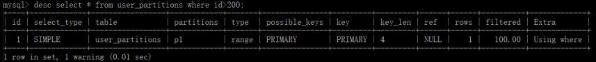
DESC SELECT * FROM user_partitions WHERE id>200;
查询id大于200(200>100,p1分区)的记录,查看执行计划,partitions是p1,符合我们的分区规则
5. type ☆
执行计划的一条记录就代表着MySQL对某个表的 执行查询时的访问方法 , 又称“访问类型”,其中的 type 列就表明了这个访问方法是啥,是较为重要的一个指标。比如,看到type列的值是ref,表明MySQL即将使用ref访问方法来执行对s1表的查询。
完整的访问方法如下: system , const , eq_ref , ref , fulltext , ref_or_null , index_merge , unique_subquery , index_subquery , range , index , ALL 。
我们详细解释一下:
-
system当表中
只有一条记录并且该表使用的存储引擎的统计数据是精确的,比如MyISAM、Memory,那么对该表的访问方法就是system。比方说我们新建一个MyISAM表,并为其插入一条记录:CREATE TABLE t(i int) Engine=MyISAM; INSERT INTO t VALUES(1);然后我们看一下查询这个表的执行计划:
EXPLAIN SELECT * FROM t;
| id | select_type | table | partitions | type | possible_keys | key | key_len | ref | rows | filtered | Extra |
|---|---|---|---|---|---|---|---|---|---|---|---|
| 1 | SIMPLE | t | null | system | null | null | null | null | 1 | 100 | null |
可以看到type列的值就是system了,
测试,可以把表改成使用InnoDB存储引擎,试试看执行计划的
type列是什么。ALL
-
const当我们根据主键或者唯一二级索引列与常数进行等值匹配时,对单表的访问方法就是
const, 比如:EXPLAIN SELECT * FROM s1 WHERE id = 10005;
| id | select_type | table | partitions | type | possible_keys | key | key_len | ref | rows | filtered | Extra |
|---|---|---|---|---|---|---|---|---|---|---|---|
| 1 | SIMPLE | s1 | null | const | PRIMARY | PRIMARY | 4 | const | 1 | 100 | null |
-
eq_ref在连接查询时,如果被驱动表是通过主键或者唯一二级索引列等值匹配的方式进行访问的(如果该主键或者唯一二级索引是联合索引的话,所有的索引列都必须进行等值比较)。则对该被驱动表的访问方法就是
eq_ref,比方说:EXPLAIN SELECT * FROM s1 INNER JOIN s2 ON s1.id = s2.id;
| id | select_type | table | partitions | type | possible_keys | key | key_len | ref | rows | filtered | Extra |
|---|---|---|---|---|---|---|---|---|---|---|---|
| 1 | SIMPLE | s1 | null | ALL | PRIMARY | null | null | null | 9895 | 100 | null |
| 1 | SIMPLE | s2 | null | eq_ref | PRIMARY | PRIMARY | 4 | atguigudb1.s1.id | 1 | 100 | null |
从执行计划的结果中可以看出,MySQL打算将s2作为驱动表,s1作为被驱动表,重点关注s1的访问 方法是 eq_ref ,表明在访问s1表的时候可以 通过主键的等值匹配 来进行访问。
-
ref当通过普通的二级索引列与常量进行等值匹配时来查询某个表,那么对该表的访问方法就可能是
ref,比方说下边这个查询:EXPLAIN SELECT * FROM s1 WHERE key1 = 'a';
| id | select_type | table | partitions | type | possible_keys | key | key_len | ref | rows | filtered | Extra |
|---|---|---|---|---|---|---|---|---|---|---|---|
| 1 | SIMPLE | s1 | null | ref | idx_key1 | idx_key1 | 303 | const | 1 | 100 | null |
-
fulltext全文索引
-
ref_or_null当对普通二级索引进行等值匹配查询,该索引列的值也可以是
NULL值时,那么对该表的访问方法就可能是ref_or_null,比如说:EXPLAIN SELECT * FROM s1 WHERE key1 = 'a' OR key1 IS NULL;
| id | select_type | table | partitions | type | possible_keys | key | key_len | ref | rows | filtered | Extra |
|---|---|---|---|---|---|---|---|---|---|---|---|
| 1 | SIMPLE | s1 | null | ref_or_null | idx_key1 | idx_key1 | 303 | const | 2 | 100 | Using index condition |
-
index_merge一般情况下对于某个表的查询只能使用到一个索引,但单表访问方法时在某些场景下可以使用
Interseation、union、Sort-Union这三种索引合并的方式来执行查询。我们看一下执行计划中是怎么体现MySQL使用索引合并的方式来对某个表执行查询的:EXPLAIN SELECT * FROM s1 WHERE key1 = 'a' OR key3 = 'a';
| id | select_type | table | partitions | type | possible_keys | key | key_len | ref | rows | filtered | Extra |
|---|---|---|---|---|---|---|---|---|---|---|---|
| 1 | SIMPLE | s1 | null | index_merge | idx_key1,idx_key3 | idx_key1,idx_key3 | 303,303 | null | 2 | 100 | Using union(idx_key1,idx_key3); Using where |
从执行计划的 type 列的值是 index_merge 就可以看出,MySQL 打算使用索引合并的方式来执行 对 s1 表的查询。
-
unique_subquery类似于两表连接中被驱动表的
eq_ref访问方法,unique_subquery是针对在一些包含IN子查询的查询语句中,如果查询优化器决定将IN子查询转换为EXISTS子查询,而且子查询可以使用到主键进行等值匹配的话,那么该子查询执行计划的type列的值就是unique_subquery,比如下边的这个查询语句:EXPLAIN SELECT * FROM s1 WHERE key2 IN (SELECT id FROM s2 where s1.key1 = s2.key1) OR key3 = 'a';
| id | select_type | table | partitions | type | possible_keys | key | key_len | ref | rows | filtered | Extra |
|---|---|---|---|---|---|---|---|---|---|---|---|
| 1 | PRIMARY | s1 | null | ALL | idx_key3 | null | null | null | 9895 | 100 | Using where |
| 2 | DEPENDENT SUBQUERY | s2 | null | unique_subquery | PRIMARY,idx_key1 | PRIMARY | 4 | func | 1 | 10 | Using where |
-
index_subqueryindex_subquery与unique_subquery类似,只不过访问子查询中的表时使用的是普通的索引 -
rangeEXPLAIN SELECT * FROM s1 WHERE key1 IN ('a', 'b', 'c');
| id | select_type | table | partitions | type | possible_keys | key | key_len | ref | rows | filtered | Extra |
|---|---|---|---|---|---|---|---|---|---|---|---|
| 1 | SIMPLE | s1 | null | range | idx_key1 | idx_key1 | 303 | null | 3 | 100 | Using index condition |
或者:
EXPLAIN SELECT * FROM s1 WHERE key1 > 'a' AND key1 < 'b';
| id | select_type | table | partitions | type | possible_keys | key | key_len | ref | rows | filtered | Extra |
|---|---|---|---|---|---|---|---|---|---|---|---|
| 1 | SIMPLE | s1 | null | range | idx_key1 | idx_key1 | 303 | null | 399 | 100 | Using index condition |
-
index当我们可以使用索引覆盖,但需要扫描全部的索引记录时,该表的访问方法就是
index,比如这样:EXPLAIN SELECT key_part2 FROM s1 WHERE key_part3 = 'a';
| id | select_type | table | partitions | type | possible_keys | key | key_len | ref | rows | filtered | Extra |
|---|---|---|---|---|---|---|---|---|---|---|---|
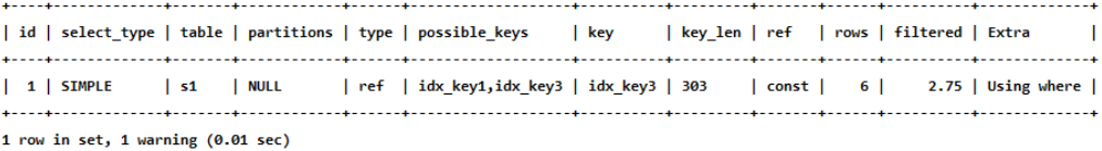
| 1 | SIMPLE | s1 | null | index | idx_key_part | idx_key_part | 909 | null | 9895 | 10 | Using where; Using index |
上述查询中的所有列表中只有key_part2 一个列,而且搜索条件中也只有 key_part3 一个列,这两个列又恰好包含在idx_key_part这个索引中,可是搜索条件key_part3不能直接使用该索引进行ref和range方式的访问,只能扫描整个idx_key_part索引的记录,所以查询计划的type列的值就是index。
再一次强调,对于使用InnoDB存储引擎的表来说,二级索引的记录只包含索引列和主键列的值,而聚簇索引中包含用户定义的全部列以及一些隐藏列,所以扫描二级索引的代价比直接全表扫描,也就是扫描聚簇索引的代价更低一些。
-
ALL最熟悉的全表扫描,就不多说了,直接看例子:
EXPLAIN SELECT * FROM s1;
| id | select_type | table | partitions | type | possible_keys | key | key_len | ref | rows | filtered | Extra |
|---|---|---|---|---|---|---|---|---|---|---|---|
| 1 | SIMPLE | s1 | null | ALL | null | null | null | null | 9895 | 100 | null |
小结:
结果值从最好到最坏依次是:
system > const > eq_ref > ref > fulltext > ref_or_null > index_merge > unique_subquery > index_subquery > range > index > ALL
其中比较重要的几个提取出来(见上图中的粗体)。SQL 性能优化的目标:至少要达到 range 级别,要求是 ref 级别,最好是 consts级别。(阿里巴巴 开发手册要求)
6. possible_keys和key
在EXPLAIN语句输出的执行计划中,possible_keys列表示在某个查询语句中,对某个列执行单表查询时可能用到的索引有哪些。一般查询涉及到的字段上若存在索引,则该索引将被列出,但不一定被查询使用。key列表示实际用到的索引有哪些,如果为NULL,则没有使用索引。比方说下面这个查询:
EXPLAIN SELECT * FROM s1 WHERE key1 > 'z' AND key3 = 'a';
上述执行计划的possible_keys列的值是idx_key1, idx_key3,表示该查询可能使用到idx_key1, idx_key3两个索引,然后key列的值是idx_key3,表示经过查询优化器计算使用不同索引的成本后,最后决定采用idx_key3。
7. key_len ☆
实际使用到的索引长度 (即:字节数)
帮你检查是否充分的利用了索引,值越大越好,主要针对于联合索引,有一定的参考意义。
EXPLAIN SELECT * FROM s1 WHERE id = 10005;
| id | select_type | table | partitions | type | possible_keys | key | key_len | ref | rows | filtered | Extra |
|---|---|---|---|---|---|---|---|---|---|---|---|
| 1 | SIMPLE | s1 | null | const | PRIMARY | PRIMARY | 4 | const | 1 | 100 | null |
int 占用 4 个字节
EXPLAIN SELECT * FROM s1 WHERE key2 = 10126;
| id | select_type | table | partitions | type | possible_keys | key | key_len | ref | rows | filtered | Extra |
|---|---|---|---|---|---|---|---|---|---|---|---|
| 1 | SIMPLE | s1 | null | const | idx_key2 | idx_key2 | 5 | const | 1 | 100 | null |
key2上有一个唯一性约束,是否为NULL占用一个字节,那么就是5个字节
mysql> EXPLAIN SELECT * FROM s1 WHERE key1 = 'a';
| id | select_type | table | partitions | type | possible_keys | key | key_len | ref | rows | filtered | Extra |
|---|---|---|---|---|---|---|---|---|---|---|---|
| 1 | SIMPLE | s1 | null | ref | idx_key1 | idx_key1 | 303 | const | 1 | 100 | null |
key1 VARCHAR(100) 一个字符占3个字节,100*3,是否为NULL占用一个字节,varchar的长度信息占两个字节。
EXPLAIN SELECT * FROM s1 WHERE key_part1 = 'a';
| id | select_type | table | partitions | type | possible_keys | key | key_len | ref | rows | filtered | Extra |
|---|---|---|---|---|---|---|---|---|---|---|---|
| 1 | SIMPLE | s1 | null | ref | idx_key_part | idx_key_part | 303 | const | 1 | 100 | null |
EXPLAIN SELECT * FROM s1 WHERE key_part1 = 'a' AND key_part2 = 'b';
| id | select_type | table | partitions | type | possible_keys | key | key_len | ref | rows | filtered | Extra |
|---|---|---|---|---|---|---|---|---|---|---|---|
| 1 | SIMPLE | s1 | null | ref | idx_key_part | idx_key_part | 606 | const,const | 1 | 100 | null |
联合索引中可以比较,key_len=606的好于key_len=303
练习:
key_len的长度计算公式:
varchar(10)变长字段且允许NULL = 10 * ( character set:utf8=3,gbk=2,latin1=1)+1(NULL)+2(变长字段)
varchar(10)变长字段且不允许NULL = 10 * ( character set:utf8=3,gbk=2,latin1=1)+2(变长字段)
char(10)固定字段且允许NULL = 10 * ( character set:utf8=3,gbk=2,latin1=1)+1(NULL)
char(10)固定字段且不允许NULL = 10 * ( character set:utf8=3,gbk=2,latin1=1)
8. ref
显示索引的哪一列被使用了,如果可能的话,是一个常数。哪些列或常量被用于查找索引列上的值.当使用索引列等值匹配的条件去执行查询时,也就是在访问方法是 const、eq_ref、ref、ref_or_nul1、unique_subquery、index_subquery其中之一时,ref列展示的就是与索引列作等值匹配的结构是什么,比如只是一个常数或者是某个列。
EXPLAIN SELECT * FROM s1 WHERE key1 = 'a';
| id | select_type | table | partitions | type | possible_keys | key | key_len | ref | rows | filtered | Extra |
|---|---|---|---|---|---|---|---|---|---|---|---|
| 1 | SIMPLE | s1 | null | ref | idx_key1 | idx_key1 | 303 | const | 1 | 100 | null |
可以看到ref列的值是const,表明在使用idx_key1索引执行查询时,与key1列作等值匹配的对象是一个常数,当然有时候更复杂一点:
EXPLAIN SELECT * FROM s1 INNER JOIN s2 ON s1.id = s2.id;
| id | select_type | table | partitions | type | possible_keys | key | key_len | ref | rows | filtered | Extra |
|---|---|---|---|---|---|---|---|---|---|---|---|
| 1 | SIMPLE | s1 | null | ALL | PRIMARY | null | null | null | 9895 | 100 | null |
| 1 | SIMPLE | s2 | null | eq_ref | PRIMARY | PRIMARY | 4 | atguigudb1.s1.id | 1 | 100 | null |
EXPLAIN SELECT * FROM s1 INNER JOIN s2 ON s2.key1 = UPPER(s1.key1);
| id | select_type | table | partitions | type | possible_keys | key | key_len | ref | rows | filtered | Extra |
|---|---|---|---|---|---|---|---|---|---|---|---|
| 1 | SIMPLE | s1 | null | ALL | null | null | null | null | 9895 | 100 | null |
| 1 | SIMPLE | s2 | null | ref | idx_key1 | idx_key1 | 303 | func | 1 | 100 | Using index condition |
9. rows ☆
预估的需要读取的记录条数,值越小越好。
EXPLAIN SELECT * FROM s1 WHERE key1 > 'z';
| id | select_type | table | partitions | type | possible_keys | key | key_len | ref | rows | filtered | Extra |
|---|---|---|---|---|---|---|---|---|---|---|---|
| 1 | SIMPLE | s1 | null | range | idx_key1 | idx_key1 | 303 | null | 384 | 100 | Using index condition |
10. filtered
某个表经过搜索条件过滤后剩余记录条数的百分比
如果使用的是索引执行的单表扫描,那么计算时需要估计出满足除使用到对应索引的搜索条件外的其他搜索条件的记录有多少条。
EXPLAIN SELECT * FROM s1 WHERE key1 > 'z' AND common_field = 'a';
| id | select_type | table | partitions | type | possible_keys | key | key_len | ref | rows | filtered | Extra |
|---|---|---|---|---|---|---|---|---|---|---|---|
| 1 | SIMPLE | s1 | null | range | idx_key1 | idx_key1 | 303 | null | 384 | 10 | Using index condition; Using where |
对于单表查询来说,这个filtered的值没有什么意义,我们更关注在连接查询中驱动表对应的执行计划记录的filtered值,它决定了被驱动表要执行的次数 (即: rows * filtered)
EXPLAIN SELECT * FROM s1 INNER JOIN s2 ON s1.key1 = s2.key1 WHERE s1.common_field = 'a';
| id | select_type | table | partitions | type | possible_keys | key | key_len | ref | rows | filtered | Extra |
|---|---|---|---|---|---|---|---|---|---|---|---|
| 1 | SIMPLE | s1 | null | ALL | idx_key1 | null | null | null | 9895 | 10 | Using where |
| 1 | SIMPLE | s2 | null | ref | idx_key1 | idx_key1 | 303 | atguigudb1.s1.key1 | 1 | 100 | null |
从执行计划中可以看出来,查询优化器打算把s1作为驱动表,s2当做被驱动表。我们可以看到驱动表s1表的执行计划的rows列为9688,filtered列为10.00,这意味着驱动表s1的扇出值就是9688 x 10.00% = 968.8,这说明还要对被驱动表执行大约968次查询。
11. Extra ☆
顾名思义,Extra列是用来说明一些额外信息的,包含不适合在其他列中显示但十分重要的额外信息。我们可以通过这些额外信息来更准确的理解MySQL到底将如何执行给定的查询语句。MySQL提供的额外信息有好几十个,我们就不一个一个介绍了,所以我们只挑选比较重要的额外信息介绍给大家。
-
No tables used当查询语句没有
FROM子句时将会提示该额外信息,比如:EXPLAIN SELECT 1;
| id | select_type | table | partitions | type | possible_keys | key | key_len | ref | rows | filtered | Extra |
|---|---|---|---|---|---|---|---|---|---|---|---|
| 1 | SIMPLE | null | null | null | null | null | null | null | null | null | No tables used |
-
Impossible WHERE当查询语句的
WHERE子句永远为FALSE时将会提示该额外信息EXPLAIN SELECT * FROM s1 WHERE 1 != 1;
| id | select_type | table | partitions | type | possible_keys | key | key_len | ref | rows | filtered | Extra |
|---|---|---|---|---|---|---|---|---|---|---|---|
| 1 | SIMPLE | null | null | null | null | null | null | null | null | null | Impossible WHERE |
Using where
不用读取表中所有信息,仅通过索引就可以获取所需数据,这发生在对表的全部的请求列都是同一个索引的部分的时候,表示mysql服务器将在存储引擎检索行后再进行过滤。表明使用了where过滤.当我们使用全表扫描来执行对某个表的查询,并且该语句的 WHERE 子句中有针对该表的搜索条件时,在Extra列中会提示上述额外信息。比如下边这个查询:
mysql> EXPLAIN SELECT * FROM s1 WHERE common_field = 'a';
| id | select_type | table | partitions | type | possible_keys | key | key_len | ref | rows | filtered | Extra |
|---|---|---|---|---|---|---|---|---|---|---|---|
| 1 | SIMPLE | s1 | null | ALL | null | null | null | null | 9895 | 10 | Using where |
当使用索引访问来执行对某个表的查询,并且该语句的 WHERE 子句中有除了该索引包含的列之外的其他搜索条件时,在Extra列中也会提示上述额外信息。比如下边这个查询虽然使用 idx_key1 索引执行查询,但是搜索条件中除了包含 key1的搜索条件 key1 =a’,还包含common_field的搜索条件,所以Extra列会显示Using where的提示:
EXPLAIN SELECT * FROM s1 WHERE key1 = 'a' AND common_field = 'a';
| id | select_type | table | partitions | type | possible_keys | key | key_len | ref | rows | filtered | Extra |
|---|---|---|---|---|---|---|---|---|---|---|---|
| 1 | SIMPLE | s1 | null | ref | idx_key1 | idx_key1 | 303 | const | 1 | 10 | Using where |
-
No matching min/max row当查询列表处有
MIN或者MAX聚合函数,但是并没有符合WHERE子句中的搜索条件的记录时。EXPLAIN SELECT MIN(key1) FROM s1 WHERE key1 = 'abcdefg';
| id | select_type | table | partitions | type | possible_keys | key | key_len | ref | rows | filtered | Extra |
|---|---|---|---|---|---|---|---|---|---|---|---|
| 1 | SIMPLE | null | null | null | null | null | null | null | null | null | No matching min/max row |
-
Using index当我们的查询列表以及搜索条件中只包含属于某个索引的列,也就是在可以使用覆盖索引的情况下,在
Extra列将会提示该额外信息。比方说下边这个查询中只需要用到idx_key1而不需要回表操作:EXPLAIN SELECT key1 FROM s1 WHERE key1 = 'a';
| id | select_type | table | partitions | type | possible_keys | key | key_len | ref | rows | filtered | Extra |
|---|---|---|---|---|---|---|---|---|---|---|---|
| 1 | SIMPLE | s1 | null | ref | idx_key1 | idx_key1 | 303 | const | 1 | 100 | Using index |
-
Using index condition有些搜索条件中虽然出现了索引列,但却不能使用到索引,比如下边这个查询:
SELECT * FROM s1 WHERE key1 > 'z' AND key1 LIKE '%a';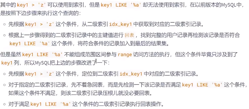
我们说回表操作其实是一个随机I0,比较耗时,所以上述修改虽然只改进了一点点,但是可以省去好多回表操作的成本。MySQL把他们的这个改进称之为索引条件下推 (英文名: Index Cndition Pushdown)如果在查询语句的执行过程中将要使用索引条件下推这个特性,在Extra列中将会显示Using index condition ,比如这样:
EXPLAIN SELECT * FROM s1 WHERE key1 > 'z' AND key1 LIKE '%b';
| id | select_type | table | partitions | type | possible_keys | key | key_len | ref | rows | filtered | Extra |
|---|---|---|---|---|---|---|---|---|---|---|---|
| 1 | SIMPLE | s1 | null | range | idx_key1 | idx_key1 | 303 | null | 384 | 100 | Using index condition |
-
Using join buffer (Block Nested Loop)在连接查询执行过程中,当被驱动表不能有效的利用索引加快访问速度,MySQL一般会为其分配一块名叫
join buffer的内存块来加快查询速度,也就是我们所讲的基于块的嵌套循环算法。EXPLAIN SELECT * FROM s1 INNER JOIN s2 ON s1.common_field = s2.common_field;
| id | select_type | table | partitions | type | possible_keys | key | key_len | ref | rows | filtered | Extra |
|---|---|---|---|---|---|---|---|---|---|---|---|
| 1 | SIMPLE | s1 | null | ALL | null | null | null | null | 9895 | 100 | null |
| 1 | SIMPLE | s2 | null | ALL | null | null | null | null | 9895 | 10 | Using where; Using join buffer (hash join) |
-
Not exists当我们使用左(外)连接时,如果
WHERE子句中包含要求被驱动表的某个列等于NULL值的搜索条件,而且那个列是不允许存储NULL值的,那么在该表的执行计划的Extra列就会提示这个信息:EXPLAIN SELECT * FROM s1 LEFT JOIN s2 ON s1.key1 = s2.key1 WHERE s2.id IS NULL;
| id | select_type | table | partitions | type | possible_keys | key | key_len | ref | rows | filtered | Extra |
|---|---|---|---|---|---|---|---|---|---|---|---|
| 1 | SIMPLE | s1 | null | ALL | null | null | null | null | 9895 | 100 | null |
| 1 | SIMPLE | s2 | null | ref | idx_key1 | idx_key1 | 303 | atguigudb1.s1.key1 | 1 | 10 | Using where; Not exists |
-
Using intersect(...) 、 Using union(...) 和 Using sort_union(...)如果执行计划的
Extra列出现了Using intersect(...)提示,说明准备使用Intersect索引合并的方式执行查询,括号中的...表示需要进行索引合并的索引名称;如果出现
Using union(...)提示,说明准备使用Union索引合并的方式执行查询;如果出现
Using sort_union(...)提示,说明准备使用Sort-Union索引合并的方式执行查询。EXPLAIN SELECT * FROM s1 WHERE key1 = 'a' OR key3 = 'a';
| id | select_type | table | partitions | type | possible_keys | key | key_len | ref | rows | filtered | Extra |
|---|---|---|---|---|---|---|---|---|---|---|---|
| 1 | SIMPLE | s1 | null | index_merge | idx_key1,idx_key3 | idx_key1,idx_key3 | 303,303 | null | 2 | 100 | Using union(idx_key1,idx_key3); Using where |
-
Zero limit当我们的
LIMIT子句的参数为0时,表示压根儿不打算从表中读取任何记录,将会提示该额外信息EXPLAIN SELECT * FROM s1 LIMIT 0;
| id | select_type | table | partitions | type | possible_keys | key | key_len | ref | rows | filtered | Extra |
|---|---|---|---|---|---|---|---|---|---|---|---|
| 1 | SIMPLE | null | null | null | null | null | null | null | null | null | Zero limit |
-
Using filesort有一些情况下对结果集中的记录进行排序是可以使用到索引的。
EXPLAIN SELECT * FROM s1 ORDER BY key1 LIMIT 10;id select_type table partitions type possible_keys key key_len ref rows filtered Extra 1 SIMPLE s1 null index null idx_key1 303 null 10 100 null 这个查询语句可以利用idx_key1 索引直接取出 key1列的10条记录,然后再进行回表操作就好了。但是很多情况下排序操作无法使用到索引,只能在内存中 (记录较少的时候)或者磁盘中(记录较多的时候)进行排序,MySQL把这种在内存中或者磁盘上进行排序的方式统称为文件排序(英文名: filesort)。如果某个查询需要使用文件排序的方式执行查询,就会在执行计划的Extra列中显示Using filesort 提示,比如这样:
EXPLAIN SELECT * FROM s1 ORDER BY common_field LIMIT 10;
| id | select_type | table | partitions | type | possible_keys | key | key_len | ref | rows | filtered | Extra |
|---|---|---|---|---|---|---|---|---|---|---|---|
| 1 | SIMPLE | s1 | null | ALL | null | null | null | null | 9895 | 100 | Using filesort |
需要注意的是,如果查询中需要使用filesort的方式进行排序的记录非常多,那么这个过程是很耗费性能的,我们最好想办法将使用文件排序的执行方式改为索引进行排序。
-
Using temporary在许多查询的执行过程中,MySQL可能会借助临时表来完成一些功能,比如去重、排序之类的,比如我们在扩行许多包含DISTINCT、GROUP BY、UNION等子句的查询过程中,如果不能有效利用索引来完成查询MySQL很有可能寻求通过建立内部的临时表来执行查询,如果查询中使用到了内部的临时表,在执行计划的Extra列将会显示Using temporary提示,比方说这样:
EXPLAIN SELECT DISTINCT common_field FROM s1;
| id | select_type | table | partitions | type | possible_keys | key | key_len | ref | rows | filtered | Extra |
|---|---|---|---|---|---|---|---|---|---|---|---|
| 1 | SIMPLE | s1 | null | ALL | null | null | null | null | 9895 | 100 | Using temporary |
再比如:
EXPLAIN SELECT common_field, COUNT(*) AS amount FROM s1 GROUP BY common_field;
| id | select_type | table | partitions | type | possible_keys | key | key_len | ref | rows | filtered | Extra |
|---|---|---|---|---|---|---|---|---|---|---|---|
| 1 | SIMPLE | s1 | null | ALL | null | null | null | null | 9895 | 100 | Using temporary |
执行计划中出现Using temporary并不是一个好的征兆,因为建立与维护临时表要付出很大的成本的,所以我们最好能使用索引来替代掉使用临时表,比方说下边这个包含GROUP BY子句的查询就不需要使用临时表:
EXPLAIN SELECT key1, COUNT(*) AS amount FROM s1 GROUP BY key1;
| id | select_type | table | partitions | type | possible_keys | key | key_len | ref | rows | filtered | Extra |
|---|---|---|---|---|---|---|---|---|---|---|---|
| 1 | SIMPLE | s1 | null | index | idx_key1 | idx_key1 | 303 | null | 9895 | 100 | Using index |
从 Extra 的 Using index 的提示里我们可以看出,上述查询只需要扫描 idx_key1 索引就可以搞 定了,不再需要临时表了。
-
其他
其它特殊情况这里省略。
12. 小结
- EXPLAIN不考虑各种Cache
- EXPLAIN不能显示MySQL在执行查询时所作的优化工作
- EXPLAIN不会告诉你关于触发器、存储过程的信息或用户自定义函数对查询的影响情况
- 部分统计信息是估算的,并非精确值
7. EXPLAIN的进一步使用
7.1 EXPLAIN四种输出格式
这里谈谈EXPLAIN的输出格式。EXPLAIN可以输出四种格式: 传统格式 ,JSON格式 , TREE格式 以及 可视化输出 。用户可以根据需要选择适用于自己的格式。
1. 传统格式
传统格式简单明了,输出是一个表格形式,概要说明查询计划。⬆️
2. JSON格式
第1种格式中介绍的EXPLAIN语句输出中缺少了一个衡量执行好坏的重要属性 —— 成本。而JSON格式是四种格式里面输出信息最详尽的格式,里面包含了执行的成本信息。
- JSON格式:在EXPLAIN单词和真正的查询语句中间加上 FORMAT=JSON 。
EXPLAIN FORMAT=JSON SELECT ....
-
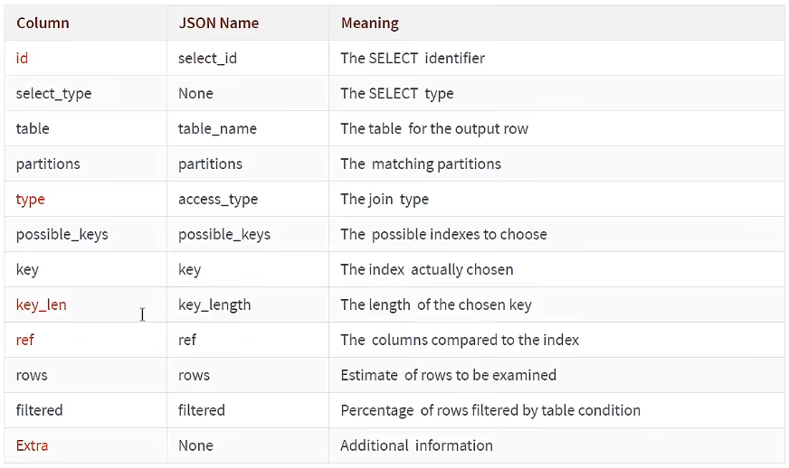
EXPLAIN的Column与JSON的对应关系:(来源于MySQL 5.7文档)
这样我们就可以得到一个json格式的执行计划,里面包含该计划花费的成本。比如这样:
EXPLAIN FORMAT=JSON SELECT * FROM s1 INNER JOIN s2 ON s1.key1 = s2.key2 WHERE s1.common_field = 'a'\G
{


  "query_block": {


    "select_id": 1,	# 整个查询语句只有1个SELECT关键字,对应id为1
    "cost_info": {


      "query_cost": "1360.07"	# 执行成本
    },
    "nested_loop": [
      # 以下是参与嵌套循环连接算法的各个表的信息
      {


        "table": {


          "table_name": "s1",	# s1驱动表
          "access_type": "ALL",	# 访问方法ALL全表扫描
          "possible_keys": [	# 可能使用的索引
            "idx_key1"
          ],
          "rows_examined_per_scan": 9895,	# 查询一次s1表大致需要扫描记录数
          "rows_produced_per_join": 989,	# 驱动表s1点扇出值
          "filtered": "10.00",						# condition filtering 条件过滤百分比
          "cost_info": {


            "read_cost": "914.80",
            "eval_cost": "98.95",
            "prefix_cost": "1013.75",		# 单次查询s1表总成本
            "data_read_per_join": "1M"	# 读取数据量
          },
          "used_columns": [		# 执行查询中涉及的列
            "id",
            "key1",
            "key2",
            "key3",
            "key_part1",
            "key_part2",
            "key_part3",
            "common_field"
          ],
          # 对s1表访问时针对单表查询的条件
          "attached_condition": "((`atguigudb1`.`s1`.`common_field` = 'a') and (`atguigudb1`.`s1`.`key1` is not null))"
        }
      },
      {


        "table": {


          "table_name": "s2",	# s2被驱动表
          "access_type": "eq_ref",	# 访问方法 等值匹配
          "possible_keys": [	# 可能使用的索引
            "idx_key2"
          ],
          "key": "idx_key2",
          "used_key_parts": [	# 实际使用的索引
            "key2"
          ],
          "key_length": "5",	# key_len
          "ref": [						# 于key2进行等值匹配的对象
            "atguigudb1.s1.key1"
          ],
          "rows_examined_per_scan": 1,		# 查询一次s2表大致需要扫描1条记录
          "rows_produced_per_join": 989,	# 被驱动表s2点扇出是968(由于后面没有多余的表进行连接,这个值也没啥用)
          "filtered": "100.00",						# condition filtering 条件过滤百分比
           # s2表使用索引进行查询的搜索条件
          "index_condition": "(cast(`atguigudb1`.`s1`.`key1` as double) = cast(`atguigudb1`.`s2`.`key2` as double))",
          "cost_info": {


            "read_cost": "247.38",
            "eval_cost": "98.95",
            "prefix_cost": "1360.08",		# 单次查询s1、多次查询s2表总成本
            "data_read_per_join": "1M"	# 读取的数据量
          },
          "used_columns": [			# 执行查询中涉及到的列
            "id",
            "key1",
            "key2",
            "key3",
            "key_part1",
            "key_part2",
            "key_part3",
            "common_field"
          ]
        }
      }
    ]
  }
}
我们使用 # 后边跟随注释的形式为大家解释了 EXPLAIN FORMAT=JSON 语句的输出内容,但是大家可能 有疑问 “cost_info” 里边的成本看着怪怪的,它们是怎么计算出来的?先看 s1 表的 “cost_info” 部 分:
"cost_info": {"read_cost": "1840.84","eval_cost": "193.76","prefix_cost": "2034.60","data_read_per_join": "1M"
}
-
read_cost是由下边这两部分组成的:- IO 成本
- 检测 rows × (1 - filter) 条记录的 CPU 成本
小贴士: rows和filter都是我们前边介绍执行计划的输出列,在JSON格式的执行计划中,rows 相当于rows_examined_per_scan,filtered名称不变。
-
eval_cost是这样计算的:检测 rows × filter 条记录的成本。
-
prefix_cost就是单独查询 s1 表的成本,也就是:read_cost + eval_cost -
data_read_per_join表示在此次查询中需要读取的数据量。
对于 s2 表的 “cost_info” 部分是这样的:
"cost_info": {"read_cost": "968.80","eval_cost": "193.76","prefix_cost": "3197.16","data_read_per_join": "1M"
}
由于 s2 表是被驱动表,所以可能被读取多次,这里的read_cost 和 eval_cost 是访问多次 s2 表后累加起来的值,大家主要关注里边儿的 prefix_cost 的值代表的是整个连接查询预计的成本,也就是单次查询 s1 表和多次查询 s2 表后的成本的和,也就是:
968.80 + 193.76 + 2034.60 = 3197.16
3. TREE格式
TREE格式是8.0.16版本之后引入的新格式,主要根据查询的 各个部分之间的关系 和 各部分的执行顺序 来描述如何查询。
EXPLAIN FORMAT=tree SELECT * FROM s1 INNER JOIN s2 ON s1.key1 = s2.key2 WHERE s1.common_field = 'a';
-> Nested loop inner join  (cost=1360.08 rows=990)
    -> Filter: ((s1.common_field = 'a') and (s1.key1 is not null))  (cost=1013.75 rows=990)
        -> Table scan on s1  (cost=1013.75 rows=9895)
    -> Single-row index lookup on s2 using idx_key2 (key2=s1.key1), with index condition: (cast(s1.key1 as double) = cast(s2.key2 as double))  (cost=0.25 rows=1)
4. 可视化输出
可视化输出,可以通过MySQL Workbench可视化查看MySQL的执行计划。通过点击Workbench的放大镜图标,即可生成可视化的查询计划。
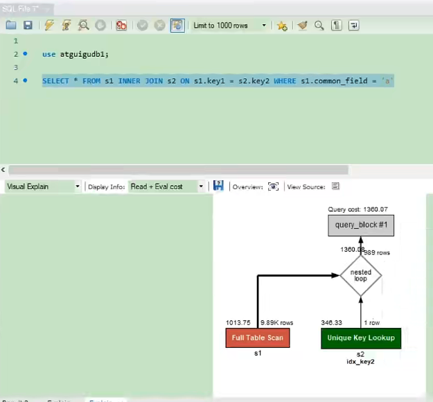
上图按从左到右的连接顺序显示表。红色框表示 全表扫描 ,而绿色框表示使用 索引查找 。对于每个表, 显示使用的索引。还要注意的是,每个表格的框上方是每个表访问所发现的行数的估计值以及访问该表的成本。
7.2 SHOW WARNINGS的使用
在我们使用EXPLAIN语句查看了某个查询的执行计划后,紧接着还可以使用SHOW WARNINGS语句查看与这个查询的执行计划有关的一些扩展信息,比如这样:
EXPLAIN SELECT s1.key1, s2.key1 FROM s1 LEFT JOIN s2 ON s1.key1 = s2.key1 WHERE s2.common_field IS NOT NULL;
SHOW WARNINGS;

/* select#1 */ select `atguigudb1`.`s1`.`key1` AS `key1`,`atguigudb1`.`s2`.`key1` AS `key1` from `atguigudb1`.`s1` join `atguigudb1`.`s2` where ((`atguigudb1`.`s1`.`key1` = `atguigudb1`.`s2`.`key1`) and (`atguigudb1`.`s2`.`common_field` is not null))
大家可以看到SHOW WARNINGS展示出来的信息有三个字段,分别是Level、Code、Message。我们最常见的就是Code为1003的信息,当Code值为1003时,Message字段展示的信息类似于查询优化器将我们的查询语句重写后的语句。比如我们上边的查询本来是一个左(外)连接查询,但是有一个s2.common_field IS NOT NULL的条件,这就会导致查询优化器把左(外)连接查询优化为内连接查询,从SHOW WARNINGS的Message字段也可以看出来,原本的LEFE JOIN已经变成了JOIN。
但是大家一定要注意,我们说Message字段展示的信息类似于查询优化器将我们的查询语句重写后的语句,并不是等价于,也就是说Message字段展示的信息并不是标准的查询语句,在很多情况下并不能直接拿到黑框框中运行,它只能作为帮助我们理解MySQL将如何执行查询语句的一个参考依据而已。
8. 分析优化器执行计划:trace
OPTIMIZER_TRACE 是MySQL 5.6引入的一项跟踪功能,它可以跟踪优化器做出的各种决策(比如访问表的方法各种开销计算、各种转换等),并将跟踪结果记录到 INFORMATION_SCHEMA.OPTIMIZER_TRACE 表中
此功能默认关闭。开启trace,并设置格式为JSON,同时设置trace最大能够使用的内存大小,避免解析过程中因为默认内存过小而不能够完整展示。
SET optimizer_trace="enabled=on",end_markers_in_json=on;
set optimizer_trace_max_mem_size=1000000;
开启后,可分析如下语句:
- SELECT
- INSERT
- REPLACE
- UPDATE
- DELETE
- EXPLAIN
- SET
- DECLARE
- CASE
- IF
- RETURN
- CALL
测试:执行如下SQL语句
select * from student where id < 10;
最后, 查询 information_schema.optimizer_trace 就可以知道MySQL是如何执行SQL的 :
select * from information_schema.optimizer_trace\G
*************************** 1. row ***************************
//第1部分:查询语句
QUERY: select * from student where id < 10
//第2部分:QUERY字段对应语句的跟踪信息
TRACE: {
"steps": [
{

   "join_preparation": { //预备工作"select#": 1,"steps": [{"expanded_query": "/* select#1 */ select `student`.`id` AS`id`,`student`.`stuno` AS `stuno`,`student`.`name` AS `name`,`student`.`age` AS`age`,`student`.`classId` AS `classId` from `student` where (`student`.`id` < 10)"}] /* steps */} /* join_preparation */
},
{

   "join_optimization": { //进行优化"select#": 1,"steps": [{"condition_processing": { //条件处理"condition": "WHERE","original_condition": "(`student`.`id` < 10)","steps": [{"transformation": "equality_propagation","resulting_condition": "(`student`.`id` < 10)"},{"transformation": "constant_propagation","resulting_condition": "(`student`.`id` < 10)"},{"transformation": "trivial_condition_removal","resulting_condition": "(`student`.`id` < 10)"}] /* steps */} /* condition_processing */},{"substitute_generated_columns": { //替换生成的列} /* substitute_generated_columns */},{"table_dependencies": [ //表的依赖关系{"table": "`student`","row_may_be_null": false,"map_bit": 0,"depends_on_map_bits": [] /* depends_on_map_bits */}] /* table_dependencies */},{"ref_optimizer_key_uses": [ //使用键] /* ref_optimizer_key_uses */},{"rows_estimation": [ //行判断{"table": "`student`","range_analysis": {"table_scan": {"rows": 3973767,"cost": 408558} /* table_scan */, //扫描表"potential_range_indexes": [ //潜在的范围索引{"index": "PRIMARY","usable": true,"key_parts": ["id"] /* key_parts */}] /* potential_range_indexes */,"setup_range_conditions": [ //设置范围条件] /* setup_range_conditions */,"group_index_range": {"chosen": false,"cause": "not_group_by_or_distinct"} /* group_index_range */,"skip_scan_range": {"potential_skip_scan_indexes": [{"index": "PRIMARY","usable": false,"cause": "query_references_nonkey_column"}] /* potential_skip_scan_indexes */} /* skip_scan_range */,"analyzing_range_alternatives": { //分析范围选项"range_scan_alternatives": [{"index": "PRIMARY","ranges": ["id < 10"] /* ranges */,"index_dives_for_eq_ranges": true,"rowid_ordered": true,"using_mrr": false,"index_only": false,"rows": 9,"cost": 1.91986,"chosen": true}] /* range_scan_alternatives */,"analyzing_roworder_intersect": {"usable": false,"cause": "too_few_roworder_scans"} /* analyzing_roworder_intersect */} /* analyzing_range_alternatives */,"chosen_range_access_summary": { //选择范围访问摘要"range_access_plan": {"type": "range_scan","index": "PRIMARY","rows": 9,"ranges": ["id < 10"] /* ranges */} /* range_access_plan */,"rows_for_plan": 9,"cost_for_plan": 1.91986,"chosen": true} /* chosen_range_access_summary */} /* range_analysis */}] /* rows_estimation */},{"considered_execution_plans": [ //考虑执行计划{"plan_prefix": [] /* plan_prefix */,"table": "`student`","best_access_path": { //最佳访问路径"considered_access_paths": [{"rows_to_scan": 9,"access_type": "range","range_details": {"used_index": "PRIMARY"} /* range_details */,"resulting_rows": 9,"cost": 2.81986,"chosen": true}] /* considered_access_paths */} /* best_access_path */,"condition_filtering_pct": 100, //行过滤百分比"rows_for_plan": 9,"cost_for_plan": 2.81986,"chosen": true}] /* considered_execution_plans */},{"attaching_conditions_to_tables": { //将条件附加到表上"original_condition": "(`student`.`id` < 10)","attached_conditions_computation": [] /* attached_conditions_computation */,"attached_conditions_summary": [ //附加条件概要{"table": "`student`","attached": "(`student`.`id` < 10)"}] /* attached_conditions_summary */} /* attaching_conditions_to_tables */},{"finalizing_table_conditions": [{"table": "`student`","original_table_condition": "(`student`.`id` < 10)","final_table_condition ": "(`student`.`id` < 10)"}] /* finalizing_table_conditions */},{"refine_plan": [ //精简计划{"table": "`student`"}] /* refine_plan */}] /* steps */} /* join_optimization */
},{

   "join_execution": { //执行"select#": 1,"steps": [] /* steps */} /* join_execution */}] /* steps */
}
//第3部分:跟踪信息过长时,被截断的跟踪信息的字节数。
MISSING_BYTES_BEYOND_MAX_MEM_SIZE: 0 //丢失的超出最大容量的字节
//第4部分:执行跟踪语句的用户是否有查看对象的权限。当不具有权限时,该列信息为1且TRACE字段为空,一般在
调用带有SQL SECURITY DEFINER的视图或者是存储过程的情况下,会出现此问题。
INSUFFICIENT_PRIVILEGES: 0 //缺失权限
1 row in set (0.00 sec)
9. MySQL监控分析视图-sys schema
Regarding MySQL performance monitoring and problem diagnosis, we generally obtain the data we want from performance_schema. In MySQL version 5.7.7, svs schema is added, which summarizes the data in performance schema and information schema in a more understandable way. Summed up as a "graph", its purpose is to reduce the complexity of querying performance_schema and allow DBA to quickly locate problems. Let’s take a look at the monitoring tables and views in these libraries. Mastering these will have the effect of getting twice the result with half the effort in our development and operation and maintenance processes.
9.1 Sys schema view summary
- Host related: Starting with host_summary, it mainly summarizes IO delay information.
- Innodb related: Starting with innodb, it summarizes the innodb buffer information and information about transactions waiting for innodb locks.
- I/o related: Starting with io, it summarizes the waiting for I/O and I/O usage.
- Memory usage: Starting with memory, it shows the memory usage from the perspective of host, thread, event, etc.
- Connection and session information: processlist and session related views, summarizing session related information.
- Table related: The view starting with schema_table shows the statistical information of the table.
- Index information: Statistics of index usage, including redundant indexes and unused indexes.
- Statement related: Starts with statement and contains statement information for performing full table scan, using temporary tables, sorting, etc.
- User related: The view starting with user counts the file I/O and execution statement statistics used by the user.
- Waiting event related information: Starting with wait, it shows the delay of waiting events.
9.2 Sys schema view usage scenarios
Index status
#1. 查询冗余索引
select * from sys.schema_redundant_indexes;
#2. 查询未使用过的索引
select * from sys.schema_unused_indexes;
#3. 查询索引的使用情况
select index_name,rows_selected,rows_inserted,rows_updated,rows_deleted
from sys.schema_index_statistics where table_schema='dbname';
table related
# 1. 查询表的访问量
select table_schema,table_name,sum(io_read_requests+io_write_requests) as io from
sys.schema_table_statistics group by table_schema,table_name order by io desc;
# 2. 查询占用bufferpool较多的表
select object_schema,object_name,allocated,data
from sys.innodb_buffer_stats_by_table order by allocated limit 10;
# 3. 查看表的全表扫描情况
select * from sys.statements_with_full_table_scans where db='dbname';
Statement related
#1. 监控SQL执行的频率
select db,exec_count,query from sys.statement_analysis
order by exec_count desc;
#2. 监控使用了排序的SQL
select db,exec_count,first_seen,last_seen,query
from sys.statements_with_sorting limit 1;
#3. 监控使用了临时表或者磁盘临时表的SQL
select db,exec_count,tmp_tables,tmp_disk_tables,query
from sys.statement_analysis where tmp_tables>0 or tmp_disk_tables >0
order by (tmp_tables+tmp_disk_tables) desc;
IO related
#1. 查看消耗磁盘IO的文件
select file,avg_read,avg_write,avg_read+avg_write as avg_io
from sys.io_global_by_file_by_bytes order by avg_read limit 10;
Innodb related
#1. 行锁阻塞情况
select * from sys.innodb_lock_waits;
Risk reminder:
When querying through the sys library, MySOL will consume a lot of resources to collect relevant information. In severe cases, business requests may be blocked, causing failures. It is recommended In production, do not frequently query sys, performance schema, and information_schema to complete monitoring, inspection, and other tasks.
10. Summary
Query is the most frequent operation in the database. Improving the query speed can effectively improve the performance of the MySQL database. By analyzing the query statement, you can understand the execution of the query statement, find out the bottleneck of query statement execution, and optimize the query statement.