(Digital Image Processing MATLAB+Python) Chapter 10 Image Segmentation - Sections 1 and 2: Threshold Segmentation and Boundary Segmentation

Article directory

1: Overview of image segmentation
2: Threshold segmentation
Three: Boundary Segmentation

1: Overview of image segmentation

Image segmentation : In the research and application of images, people are often only interested in certain targets in the image, which usually correspond to areas with specific properties in the image. Image segmentation refers to an image processing technology that divides an image into different regions with specific properties, and separates and extracts these regions for further feature extraction and understanding.

Insert image description here

There are many image segmentation methods, and commonly used techniques include:

Threshold-based : Divide the image into different regions based on the gray value or color information of the pixels. This method is simple and intuitive, suitable for some simple scenes, but may not work well for complex images.
Based on edge detection : segment the image into different areas by detecting edge information in the image. Commonly used edge detection algorithms include Canny edge detection and Sobel operator, etc.
Based on region growing : Starting from seed pixels, adjacent pixels are gradually merged into a region according to certain similarity criteria until the stopping criterion is met. This method works better for images with obvious regional boundaries.
Based on graph cuts : The image segmentation problem is transformed into a graph cut problem in graph theory, and segmentation is achieved by minimizing the energy function in the graph. This method can capture the global relationship between pixels and has better accuracy.
Based on deep learning : In recent years, deep learning technology has made significant progress in image segmentation. By using a deep convolutional neural network (CNN) or a fully convolutional network (FCN), the semantic information of the image can be learned and pixel-level segmentation results can be generated.

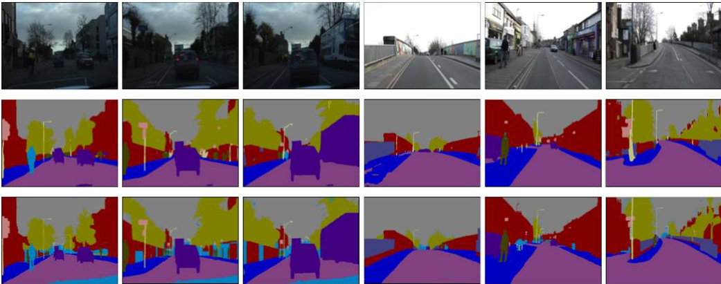
Image segmentation plays a key role in many applications. For example, in medical image processing, image segmentation can be used to identify and locate tumors or diseased areas to help doctors make diagnosis and treatment decisions. In the field of autonomous driving, image segmentation can be used to identify roads, pedestrians, traffic signs, etc., and provide key information about the environment. In addition, image segmentation is also widely used in fields such as image editing, target detection, virtual reality and augmented reality.

2: Threshold segmentation

(1 Overview

Threshold segmentation : It is one of the simplest and commonly used methods in image segmentation. It divides pixels in an image into two or more different regions based on their gray value or color information. The basic idea of threshold segmentation is to choose a threshold to divide the pixels in the image into two categories above or below the threshold. Proceed as follows

Grayscale : Convert a color image to grayscale for processing on a single grayscale channel
Select threshold : Choose an appropriate threshold to segment the image into different regions. Thresholds can be chosen based on experience, histogram analysis, adaptive methods, etc.
Segment Image : Classify pixels in an image into two or more categories based on a selected threshold. Typically, pixel values above a threshold are assigned to one category, and pixel values below the threshold are assigned to another category.

The principle of threshold segmentation is as follows

$y)=\left\{\begin{array}{ll}1 & f(x, y) \geq T \\0 & f(x, y)<T\end{array}\right.$

Among them, $f (x, y)$ is the original image, $g (x, y)$ is the result image (binary value), $T$ is the threshold. Obviously, the selection of the threshold determines the quality of the binarization effect.

(2) Thresholding

Thresholding : is a common technique in image processing used to separate pixels in an image into two or more different categories, such as dividing an image into foreground and background. Thresholding determines which category a pixel belongs to by setting a threshold based on the gray value or color information of the pixel. During thresholding, pixels are classified based on their relationship to a threshold. Typically, if a pixel value is above a threshold, it is classified into one category (e.g., foreground), otherwise it is classified into another category (e.g., background). The purpose of thresholding is to simplify or segment the image according to its characteristics to facilitate subsequent processing or analysis. Thresholding is often used in the following application scenarios

Target detection : By segmenting the image into foreground and background, it is easier to extract the target area of interest and perform subsequent target detection and recognition.
Image segmentation : Thresholding can segment images into different regions, such as segmenting tumor areas from medical images or separating objects from complex backgrounds.
Image enhancement : By choosing an appropriate threshold, certain features of the image can be enhanced, such as enhancing the edge information of the image or improving the contrast of the image.
Object counting : By dividing the pixels in the image into foreground and background, the foreground pixels can be counted to achieve an estimation or statistics of the number of objects.

There are many methods and techniques for thresholding, such as

Upper thresholding : All pixels with grayscale values greater than or equal to the threshold are regarded as foreground pixels, and the remaining pixels are regarded as background pixels.
Lower thresholding : All pixels with grayscale values less than or equal to the threshold are regarded as foreground pixels
Inner thresholding : Determine a smaller threshold and a larger threshold, and pixels with grayscale values between the two are regarded as foreground pixels.
External thresholding : pixels with grayscale values between the small threshold and the large threshold are regarded as foreground pixels

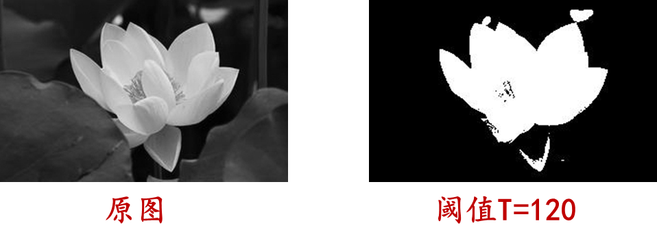
(3) Threshold selection based on grayscale histogram

A: Principle

Threshold selection based on grayscale histogram : It selects appropriate thresholds based on the grayscale distribution characteristics of the image to segment the image into different regions.

Grayscale histogram : First, calculate the grayscale histogram of the image, that is, count the number of pixels at different grayscale levels. Grayscale histogram can reflect the distribution of various grayscale levels in the image.
Threshold selection : Based on the shape and characteristics of the grayscale histogram, select an appropriate threshold to segment the image into different regions. Common threshold selection methods include the following
- Single peak threshold method : suitable for situations where the image grayscale histogram presents a single obvious peak. The threshold is usually chosen at or near the peak
- Bimodal threshold method : It is suitable for situations where the image grayscale histogram presents two obvious peaks, one of which represents the background and the other represents the target or foreground. Threshold selection is usually at the valley between two peaks
- Otsu's method : Otsu's method is an adaptive threshold selection method based on the maximum inter-class variance. It can automatically select a threshold that maximizes the inter-class variance between the foreground and background of the segmented image.
- Gaussian Mixture Model (GMM) : The GMM method assumes that the pixel gray value in the image obeys multiple Gaussian distributions. By fitting multiple Gaussian distributions, the turning point between each distribution is found as a threshold.
Segment the image : According to the selected threshold, the pixels in the image are divided into two or more categories. Usually, pixels whose grayscale value is higher than the threshold are classified into one category, and those below the threshold are classified into another category.

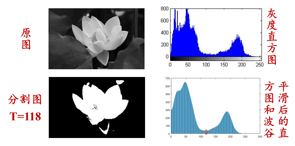
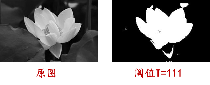
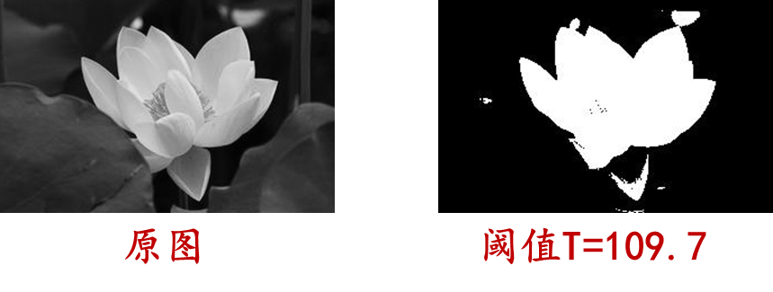
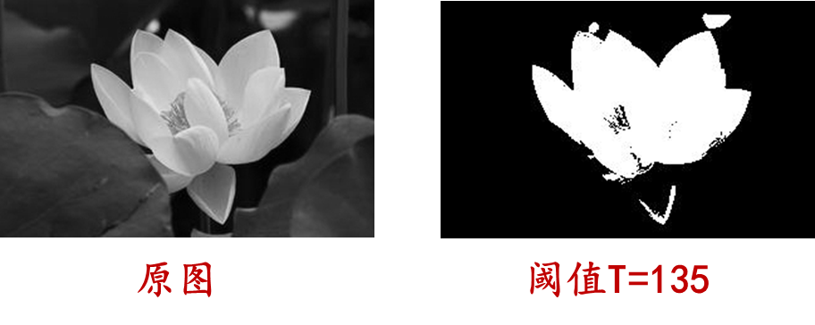
For example, in the figure below, the grayscale histogram of the image is a bimodal distribution, indicating that the content of the image is roughly divided into two parts, which are near the two peaks of the grayscale distribution. Then the threshold value is selected to be the grayscale value corresponding to the valley point between the two peaks . . This is a special method that is suitable for situations where the foreground and background grayscale differences in the image are obvious and each accounts for a certain proportion. If the overall histogram of the image does not have bimodal or multimodal characteristics, it can be considered for local application.

Insert image description here

B：Program

As follows: Implement histogram selection threshold based on bimodal distribution to segment the image

The point is to find the peaks and valleys of the histogram, but the histogram is usually not smooth, so first smooth the histogram and then search for the peaks and valleys
In the programming, the frequencies of three adjacent gray levels in the histogram are added and averaged as the frequency corresponding to the middle gray level, and the histogram is continuously smoothed until it becomes a bimodal distribution.
Other methods can also be used to determine peaks and valleys

Insert image description here

matlab implementation :

clear,clc,close all;
Image=rgb2gray(imread('lotus1.jpg'));
figure,imshow(Image),title('原始图像');
imhist(Image);
hist1=imhist(Image);
hist2=hist1;
iter=0;
while 1
    [is,peak]=Bimodal(hist1);
    if is==0
        hist2(1)=(hist1(1)*2+hist1(2))/3;
        for j=2:255
            hist2(j)=(hist1(j-1)+hist1(j)+hist1(j+1))/3;
        end
        hist2(256)=(hist1(255)+hist1(256)*2)/3;
        hist1=hist2;
        iter=iter+1;
        if iter>1000
            break;
        end
    else
        break;
    end
end

[trough,pos]=min(hist1(peak(1):peak(2)));
thresh=pos+peak(1);
figure,stem(1:256,hist1,'Marker','none');
hold on
stem([thresh,thresh],[0,trough],'Linewidth',2);
hold off
result=zeros(size(Image));
result(Image>thresh)=1;
figure,imshow(result),title('基于双峰直方图的阈值化');
imwrite(result,'bilotus1.jpg');   

function [is,peak]=Bimodal(histgram)
    count=0;
    for j=2:255
        if histgram(j-1)<histgram(j) && histgram(j+1)<histgram(j)
            count=count+1;
            peak(count)=j;
            if count>2 
                is=0;
                return;
            end
        end
    end
    if count==2
        is=1;
    else
        is=0;
    end
end

import cv2
import numpy as np
import matplotlib.pyplot as plt

def Bimodal(histgram):
    count = 0
    peak = []
    for j in range(1, 255):
        if histgram[j-1] < histgram[j] and histgram[j+1] < histgram[j]:
            count += 1
            peak.append(j)
            if count > 2:
                return 0, peak
    if count == 2:
        return 1, peak
    else:
        return 0, peak

# 读取图像并转换为灰度图像
image = cv2.imread('lotus1.jpg')
gray_image = cv2.cvtColor(image, cv2.COLOR_BGR2GRAY)

# 显示原始图像
plt.figure()
plt.imshow(gray_image, cmap='gray')
plt.title('原始图像')

# 绘制灰度直方图
plt.figure()
plt.hist(gray_image.ravel(), bins=256, color='gray')
plt.title('灰度直方图')

# 计算灰度直方图
hist1 = cv2.calcHist([gray_image], [0], None, [256], [0, 256])
hist2 = hist1.copy()
iter = 0
while True:
    is_bimodal, peak = Bimodal(hist1)
    if is_bimodal == 0:
        hist2[0] = (hist1[0]*2 + hist1[1]) / 3
        for j in range(1, 255):
            hist2[j] = (hist1[j-1] + hist1[j] + hist1[j+1]) / 3
        hist2[255] = (hist1[254] + hist1[255]*2) / 3
        hist1 = hist2
        iter += 1
        if iter > 1000:
            break
    else:
        break

# 根据双峰直方图选择阈值
trough, pos = np.min(hist1[peak[0]:peak[1]]), np.argmin(hist1[peak[0]:peak[1]])
thresh = pos + peak[0]

# 绘制带阈值的直方图
plt.figure()
plt.stem(np.arange(256), hist1, markerfmt='none')
plt.axvline(x=thresh, ymin=0, ymax=trough, linewidth=2)
plt.title('双峰直方图阈值化')

# 基于阈值进行图像分割
result = np.zeros_like(gray_image)
result[gray_image > thresh] = 255

# 显示分割结果
plt.figure()
plt.imshow(result, cmap='gray')
plt.title('基于双峰直方图的阈值化')

# 保存结果图像
cv2.imwrite('bilotus1.jpg', result)

# 显示所有图像
plt.show()

(4) Threshold selection based on pattern classification ideas

A: Principle

Threshold selection based on pattern classification ideas : It is a method of selecting thresholds based on the characteristic pattern of pixels. It is based on analyzing and classifying the characteristics of different pixels in the image to determine the optimal threshold to segment the image into different regions. The following are the basic steps for threshold selection based on pattern classification ideas.

Calculate features : First, perform feature calculations on pixels in the image. Common features include pixel grayscale values, gradients, textures, etc.
Division mode : Classify pixels according to different modes of features. Classify pixels into different pattern categories based on specific thresholds. For example, pixels can be divided into background and foreground mode categories
Calculate the difference measure between categories : Calculate the difference measure between different pattern categories, such as the average grayscale difference, variance, etc. between categories. These measures reflect the degree of separation between different categories
Select the best threshold : Based on the difference measure between categories, select the best threshold as the threshold for segmenting the image. Generally, a larger inter-category difference measure means better segmentation
Apply Threshold : Segment the image into different regions using the selected threshold. Compare pixel grayscale values with thresholds and classify pixels into different categories based on the comparison results

The threshold selection method based on pattern classification ideas can adapt to different image features and segmentation requirements. By performing feature analysis and pattern classification on pixels, this method is able to select the best threshold based on the intrinsic characteristics of the image, thereby achieving effective image segmentation. However, selecting appropriate features and a suitable pattern classification algorithm are key to this method and need to be selected and optimized according to the specific problem

B: Maximum inter-class variance method (OTSU)

Maximum inter-class variance method (OTSU) : It is an adaptive image threshold selection method used to segment the image into two areas: foreground and background. This method selects the best threshold by maximizing the inter-class variance between two categories of the image to achieve the best segmentation effect. The following is the basic principle of the maximum inter-class variance method

Calculate histogram : First, calculate the grayscale histogram of the image and count the number of pixels at different grayscale levels
Calculate the intra-class variance : For each possible threshold (0 to 255), divide the image into two categories, foreground and background, and calculate the intra-class variance for both categories. Intra-class variance reflects the degree of change in pixel gray value within the same category
Calculate inter-class variance : By segmenting the image into two categories, foreground and background, calculate the inter-class variance between these two categories. Inter-class variance reflects the degree of grayscale difference between two categories
Maximize the inter-class variance : traverse all possible thresholds and find the threshold that maximizes the inter-class variance, that is, the optimal threshold. Maximizing the inter-class variance means maximizing the difference between the foreground and background, thereby achieving the best image segmentation effect
Apply Threshold : Segment the image into two regions, foreground and background, using the chosen optimal threshold. Compare pixel grayscale values with thresholds and classify pixels into different categories based on the comparison results

Two types of variance

$\sigma_{o}^{2}=\frac{1}{p_{o}} \sum_{i=0}^{T} p_{i}\left(i-\mu_{o}\right)^{2} \quad \sigma_{B}^{2}=\frac{1}{p_{B}} \sum_{i=T+1}^{L-1} p_{i}\left(i-\mu_{B}\right)^{2}$

Within-class variance and between-class variance

$\begin{array}{l}\ sigma_{in}^{2}=p_{O} \cdot \sigma_{o}^{2}+p_{B} \cdot \sigma_{B}^{2} \\\sigma_{1}^{2 }=p_{o} \times\left(\mu_{o}-\mu\right)^{2}+p_{B} \times\left(\mu_{B}-\mu\right)^{2 }\end{array}$

as follows

Insert image description here

matlab implementation

Image=rgb2gray(imread('lotus1.jpg'));
figure,imshow(Image),title('原始图像');
T=graythresh(Image);
result=im2bw(Image,T);
figure,imshow(result),title('OTSU方法二值化图像 ');
% imwrite(result,'lotus1otsu.jpg');

python implementation :

import cv2
import numpy as np
import matplotlib.pyplot as plt

# 读取图像并转换为灰度图像
image = cv2.imread('lotus1.jpg')
gray_image = cv2.cvtColor(image, cv2.COLOR_BGR2GRAY)

# 显示原始图像
plt.figure()
plt.imshow(gray_image, cmap='gray')
plt.title('原始图像')

# 使用Otsu方法选择阈值
_, threshold = cv2.threshold(gray_image, 0, 255, cv2.THRESH_BINARY + cv2.THRESH_OTSU)

# 对图像进行二值化
result = cv2.bitwise_and(gray_image, threshold)

# 显示二值化结果
plt.figure()
plt.imshow(result, cmap='gray')
plt.title('OTSU方法二值化图像')

# 保存结果图像
# cv2.imwrite('lotus1otsu.jpg', result)

# 显示所有图像
plt.show()

C: Maximum entropy method

Maximum entropy method : It is one of the commonly used image segmentation methods, used to segment images into different regions. It is based on the concept of information entropy and selects the best segmentation result by maximizing the entropy of each region in the image. The following is the basic principle of the maximum entropy method

Define image entropy : First, calculate the global entropy of the image, that is, treat the entire image as a region and calculate its entropy. Image entropy is a measure of the randomness and uncertainty of the grayscale distribution of an image.
Define local entropy : Divide the image into different regions and calculate the local entropy of each region. Local entropy reflects the randomness and uncertainty of pixel grayscale distribution in each area.
Calculate conditional entropy : Calculate the conditional entropy of each region based on the segmentation result of the image. Conditional entropy refers to the randomness and uncertainty of the grayscale distribution of the pixels in each area when the area is segmented.
Define the objective function : Define an objective function, such as the maximum entropy criterion function, which combines global entropy, local entropy and conditional entropy. The goal of the objective function is to maximize the entropy of the segmentation result to achieve the best image segmentation effect.
Find the best segmentation : Search for the best segmentation results through iterative optimization methods or other optimization algorithms. The ultimate goal is to find the optimal region segmentation that maximizes the objective function

The maximum entropy method can adaptively select the best segmentation result of the image without knowing the characteristics or background information of the image in advance. By maximizing the entropy of the image, this method can find the best segmentation results on the boundaries between different regions, and is suitable for different types of image segmentation tasks. It should be noted that the maximum entropy method may need to consider some factors in practical applications, such as computational complexity, initial segmentation results, optimization algorithms, etc. Depending on the specific application requirements and image characteristics, other image processing technologies and algorithms may need to be combined to improve the accuracy and robustness of segmentation.

as follows

Insert image description here

matlab implementation :

clear,clc,close all;
Image=rgb2gray(imread('fruit.jpg'));
figure,imshow(Image),title('原始图像');
hist=imhist(Image);
bottom=min(Image(:))+1;
top=max(Image(:))+1;
J=zeros(256,1);
for t=bottom+1:top-1
    po=sum(hist(bottom:t));
    pb=sum(hist(t+1:top));
    ho=0;
    hb=0;
    for j=bottom:t
        ho=ho-log(hist(j)/po+0.01)*hist(j)/po;
    end
    for j=t+1:top
        hb=hb-log(hist(j)/pb+0.01)*hist(j)/pb;
    end
    J(t)=ho+hb;        
end
[maxJ,pos]=max(J(:));
result=zeros(size(Image));
result(Image>pos)=1;
figure,imshow(result);

python implementation :

import cv2
import numpy as np
import matplotlib.pyplot as plt

# 读取图像并转换为灰度图像
image = cv2.imread('fruit.jpg')
gray_image = cv2.cvtColor(image, cv2.COLOR_BGR2GRAY)

# 显示原始图像
plt.figure()
plt.imshow(gray_image, cmap='gray')
plt.title('原始图像')

# 计算图像直方图
hist = cv2.calcHist([gray_image], [0], None, [256], [0, 256])

bottom = np.min(gray_image) + 1
top = np.max(gray_image) + 1
J = np.zeros((256, 1))

for t in range(bottom + 1, top):
    po = np.sum(hist[bottom:t])
    pb = np.sum(hist[t+1:top])
    ho = 0
    hb = 0
    for j in range(bottom, t):
        ho = ho - np.log(hist[j] / po + 0.01) * hist[j] / po
    for j in range(t+1, top):
        hb = hb - np.log(hist[j] / pb + 0.01) * hist[j] / pb
    J[t] = ho + hb

maxJ, pos = np.max(J), np.argmax(J)

# 分割图像
result = np.zeros_like(gray_image)
result[gray_image > pos] = 255

# 显示分割结果
plt.figure()
plt.imshow(result, cmap='gray')

# 显示所有图像
plt.show()

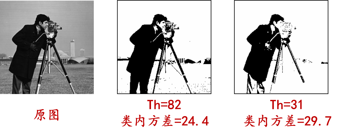
D: Minimum error method

Minimum error method : It is one of the commonly used image segmentation methods, used to segment images into different regions. It is based on the statistical properties of pixel gray values and selects the best threshold by minimizing the error in segmentation to achieve the best segmentation effect. The following is the basic principle of the minimum error method

Calculate histogram : First, calculate the grayscale histogram of the image and count the number of pixels at different grayscale levels
Initialization threshold : Choose an initial threshold, which can be a value determined based on experience, or a preliminary estimate selected based on some criterion
Calculate the average gray value : According to the current threshold, the image is divided into two areas: the area below the threshold is the background, and the area above the threshold is the foreground. Calculate the average gray value of two areas
Update threshold : Update the threshold based on the average gray value calculated in the previous step. Common update methods include taking the average or weighted average of the average gray value of two areas
Calculate error : Calculate the error in segmentation based on the updated threshold. Error can be defined according to different criteria, such as mean square error, cross entropy, etc.
Repeat steps 3 to 5 : Perform steps 3 to 5 iteratively until convergence conditions are reached, such as the change in threshold is less than a certain threshold, or the error no longer changes significantly
Optimal threshold selection : Based on the convergence results, select the best threshold as the image segmentation threshold.

The minimum error method can adaptively select the best segmentation threshold according to the gray distribution characteristics of the image. Through an iterative optimization process, this method achieves the best image segmentation effect by minimizing the error in segmentation. It should be noted that the performance of the minimum error method is affected by the choice of initial threshold and convergence conditions. Choosing an appropriate initial threshold and appropriate convergence conditions can help improve the accuracy and efficiency of segmentation. In addition, for complex image scenes, it may be necessary to combine other image processing techniques and algorithms to improve the accuracy and robustness of segmentation.

as follows

Insert image description here

matlab implementation :

clear,clc,close all;
Image=rgb2gray(imread('fruit.jpg'));
figure,imshow(Image),title('原始图像');
hist=imhist(Image);
bottom=min(Image(:))+1;
top=max(Image(:))+1; 
J=zeros(256,1);
J=J+100000;
alpha=0.25;
scope=find(hist>5);
minthresh=scope(1);
maxthresh=scope(end);
for t=minthresh+1:maxthresh-1
    miuo=0;
    sigmaho=0;
    for j=bottom:t
        miuo=miuo+hist(j)*double(j);
    end
    pixelnum=sum(hist(bottom:t));
    miuo=miuo/pixelnum;
    for j=bottom:t
        sigmaho=sigmaho+(double(j)-miuo)^2*hist(j);
    end
    sigmaho=sigmaho/pixelnum;
    
    miub=0;
    sigmahb=0;
    for j=t+1:top
        miub=miub+hist(j)*double(j);
    end
    pixelnum=sum(hist(t+1:top));
    miub=miub/pixelnum;
    for j=t+1:top
        sigmahb=sigmahb+(double(j)-miub)^2*hist(j);
    end
    sigmahb=sigmahb/pixelnum;
    
    Epsilonb=0;
    Epsilono=0;
    for j=bottom:t
        pb=exp(-(double(j)-miub)^2/(sigmahb*2+eps))/(sqrt(2*pi*sigmahb)+eps);
        Epsilonb=Epsilonb+pb;
    end
    for j=t+1:top        
        po=exp(-(double(j)-miuo)^2/(sigmaho*2+eps))/(sqrt(2*pi*sigmaho)+eps);
        Epsilono=Epsilono+po;
    end
    J(t)=alpha*Epsilono+(1-alpha)*Epsilonb;
end
[minJ,pos]=min(J(:));
result=zeros(size(Image));
result(Image>pos)=1;
figure,imshow(result),title('最小误差阈值法');

python implementation :

import cv2
import numpy as np
import matplotlib.pyplot as plt

# 读取图像并转换为灰度图像
image = cv2.imread('fruit.jpg')
image_gray = cv2.cvtColor(image, cv2.COLOR_BGR2GRAY)

# 显示原始图像
plt.figure()
plt.imshow(image_gray, cmap='gray')
plt.title('原始图像')

# 计算直方图
hist = cv2.calcHist([image_gray], [0], None, [256], [0, 256])

bottom = np.min(image_gray) + 1
top = np.max(image_gray) + 1
J = np.zeros((256, 1)) + 100000
alpha = 0.25

# 找到直方图中像素数大于5的范围
scope = np.where(hist > 5)[0]
minthresh = scope[0]
maxthresh = scope[-1]

for t in range(minthresh + 1, maxthresh):
    miuo = 0
    sigmaho = 0

    for j in range(bottom, t):
        miuo += hist[j] * j

    pixelnum = np.sum(hist[bottom:t])
    miuo /= pixelnum

    for j in range(bottom, t):
        sigmaho += (j - miuo) ** 2 * hist[j]

    sigmaho /= pixelnum

    miub = 0
    sigmahb = 0

    for j in range(t + 1, top):
        miub += hist[j] * j

    pixelnum = np.sum(hist[t + 1:top])
    miub /= pixelnum

    for j in range(t + 1, top):
        sigmahb += (j - miub) ** 2 * hist[j]

    sigmahb /= pixelnum

    Epsilonb = 0
    Epsilono = 0

    for j in range(bottom, t):
        pb = np.exp(-(j - miub) ** 2 / (sigmahb * 2 + np.finfo(float).eps)) / (np.sqrt(2 * np.pi * sigmahb) + np.finfo(float).eps)
        Epsilonb += pb

    for j in range(t + 1, top):
        po = np.exp(-(j - miuo) ** 2 / (sigmaho * 2 + np.finfo(float).eps)) / (np.sqrt(2 * np.pi * sigmaho) + np.finfo(float).eps)
        Epsilono += po

    J[t] = alpha * Epsilono + (1 - alpha) * Epsilonb

minJ, pos = np.min(J), np.argmin(J)
result = np.zeros(image_gray.shape)

# 根据阈值分割图像
result[image_gray > pos] = 1

# 显示分割结果
plt.figure()
plt.imshow(result, cmap='gray')
plt.title('最小误差阈值法')

plt.show()

(5) Other threshold segmentation methods

A: Threshold selection based on iterative operation

Threshold selection based on iterative operation : It is a commonly used image segmentation method. It uses repeated iterations to find the optimal threshold to segment the image into target and background parts. The basic idea of this method is to divide the gray value of the image into two areas according to the threshold, and update the threshold based on the average gray value of the two areas until a certain termination condition is met. The general steps are as follows

Select the initial threshold : it can be any reasonable value, such as the median value of the image gray value
Based on the selected threshold, the image is divided into two regions : one region contains pixels greater than the threshold and the other contains pixels less than or equal to the threshold
Calculate the average gray value of two areas : one is the average gray value of pixels greater than the threshold, and the other is the average gray value of the pixels less than or equal to the threshold
Use the average of the average grayscale values as the new threshold
Repeat steps 2 to 4 until a certain stopping criterion is met : Commonly used stopping criteria include that the change in the threshold is less than a certain preset threshold or the number of iterations reaches a preset value
The final threshold is the optimal threshold, and the image is binarized and segmented based on this threshold.

The threshold segmentation method based on iterative operation is simple and easy to understand, and is suitable for most images, especially for images with bimodal grayscale histogram characteristics. However, this method may not be stable and accurate enough for image noise and uneven grayscale distribution, so parameter adjustment and optimization may be required in practical applications.

as follows

Insert image description here

matlab implementation :

clear,clc,close all;
Image=im2double(rgb2gray(imread('lotus1.jpg')));
figure,imshow(Image),title('原始图像');
T=(max(Image(:))+min(Image(:)))/2;
equal=false;
while ~equal
    rb=find(Image>=T);
    ro=find(Image<T);
    NewT=(mean(Image(rb))+mean(Image(ro)))/2;
    equal=abs(NewT-T)<1/256;
    T=NewT;
end
result=im2bw(Image,T);
figure,imshow(result),title('迭代方法二值化图像 ');

python implementation :

import cv2
import numpy as np
import matplotlib.pyplot as plt

# 读取图像并转换为灰度图像
image = cv2.imread('lotus1.jpg')
image_gray = cv2.cvtColor(image, cv2.COLOR_BGR2GRAY)
image_gray = image_gray.astype(float) / 255.0

# 显示原始图像
plt.figure()
plt.imshow(image_gray, cmap='gray')
plt.title('原始图像')

# 初始化阈值
T = (np.max(image_gray) + np.min(image_gray)) / 2
equal = False

while not equal:
    rb = np.where(image_gray >= T)
    ro = np.where(image_gray < T)
    NewT = (np.mean(image_gray[rb]) + np.mean(image_gray[ro])) / 2
    equal = abs(NewT - T) < 1 / 256
    T = NewT

# 根据阈值进行二值化
result = (image_gray >= T).astype(np.uint8)

# 显示二值化结果
plt.figure()
plt.imshow(result, cmap='gray')
plt.title('迭代方法二值化图像')

plt.show()

B: Threshold selection based on fuzzy theory

Threshold selection based on fuzzy theory : Unlike the traditional binarization method that only uses a fixed threshold, the threshold segmentation method based on fuzzy theory uses fuzzy sets to describe the membership degree of pixels belonging to the target or background, thereby more flexibly processing different images in the image. Certainty and complexity. Fuzziness represents the degree of ambiguity of a fuzzy set, and fuzzy entropy is a quantitative indicator that measures ambiguity. Fuzzy entropy is used as the objective function to solve for the optimal threshold. Proceed as follows

Determine the fuzzification method : blur the original image. Common fuzzification methods include Gaussian blur, mean blur, etc. Blurring helps reduce the impact of noise and converts images into fuzzy sets
Determine the membership function : Define a membership function for each pixel in the image. The membership function describes the degree to which the pixel belongs to the target or background. Common membership functions include triangular membership functions, Gaussian membership functions, etc.
Determine the blur threshold : Choose an appropriate blur threshold to divide the pixels into targets or backgrounds based on the membership function. This process is equivalent to threshold determination in traditional binarization, but based on fuzzy theory, the threshold becomes fuzzy, allowing pixels to have fuzzy membership degrees between the target and the background.
Fuzzy inversion : According to the determined fuzzy threshold, the fuzzy set is mapped back to the binary image through fuzzy inversion to obtain the final segmentation result.

The threshold segmentation method based on fuzzy theory has stronger adaptability and robustness than the traditional binarization method, and is especially suitable for situations where there is a fuzzy boundary between the target and the background in the image. This method can perform better when processing images with noisy or uneven lighting, but may require more computing resources in some cases. Therefore, it is necessary to choose an appropriate image segmentation method according to the specific situation during application.

as follows

Insert image description here

matlab implementation :

clear,clc,close all;
Image=rgb2gray(imread('lotus1.jpg'));
figure,imshow(Image),title('原始图像');
hist=imhist(Image);
bottom=min(Image(:))+1;
top=max(Image(:))+1; 
C=double(top-bottom);
S=zeros(256,1);
J=10^10;
for t=bottom+1:top-1
    miuo=0;
    for j=bottom:t
        miuo=miuo+hist(j)*double(j);
    end
    pixelnum=sum(hist(bottom:t));
    miuo=miuo/pixelnum;
    for j=bottom:t
        miuf=1/(1+abs(double(j)-miuo)/C);
        S(j)=-miuf*log(miuf)-(1-miuf)*log(1-miuf);
    end
        
    miub=0;
    for j=t+1:top
        miub=miub+hist(j)*double(j);
    end
    pixelnum=sum(hist(t+1:top));
    miub=miub/pixelnum;
    for j=t+1:top
        miuf=1/(1+abs(double(j)-miub)/C);
        S(j)=-miuf*log(miuf)-(1-miuf)*log(1-miuf);
    end
    currentJ=sum(hist(bottom:top).*S(bottom:top));
    if currentJ<J
        J=currentJ;
        thresh=t;
    end           
end
result=zeros(size(Image));
result(Image>thresh)=1;
figure,imshow(result);

python implementation :

import cv2
import numpy as np
import matplotlib.pyplot as plt

def fuzzy_threshold_segmentation(image):
    image_gray = cv2.cvtColor(image, cv2.COLOR_BGR2GRAY)
    hist = cv2.calcHist([image_gray], [0], None, [256], [0, 256])
    bottom = np.min(image_gray) + 1
    top = np.max(image_gray) + 1
    C = float(top - bottom)
    S = np.zeros(256)
    J = 10**10
    for t in range(int(bottom + 1), int(top)):
        miuo = 0
        for j in range(int(bottom), int(t)):
            miuo += hist[j] * float(j)
        pixelnum = np.sum(hist[int(bottom):int(t)])
        miuo = miuo / pixelnum
        for j in range(int(bottom), int(t)):
            miuf = 1 / (1 + abs(float(j) - miuo) / C)
            S[j] = -miuf * np.log(miuf) - (1 - miuf) * np.log(1 - miuf)

        miub = 0
        for j in range(int(t + 1), int(top)):
            miub += hist[j] * float(j)
        pixelnum = np.sum(hist[int(t + 1):int(top)])
        miub = miub / pixelnum
        for j in range(int(t + 1), int(top)):
            miuf = 1 / (1 + abs(float(j) - miub) / C)
            S[j] = -miuf * np.log(miuf) - (1 - miuf) * np.log(1 - miuf)

        currentJ = np.sum(hist[int(bottom):int(top)] * S[int(bottom):int(top)])
        if currentJ < J:
            J = currentJ
            thresh = t

    result = np.zeros_like(image_gray)
    result[image_gray > thresh] = 255
    return result

if __name__ == "__main__":
    image = cv2.imread('lotus1.jpg')
    segmented_image = fuzzy_threshold_segmentation(image)

    plt.figure()
    plt.subplot(1, 2, 1)
    plt.imshow(cv2.cvtColor(image, cv2.COLOR_BGR2RGB))
    plt.title('原始图像')
    plt.subplot(1, 2, 2)
    plt.imshow(segmented_image, cmap='gray')
    plt.title('分割结果')
    plt.show()

Three: Boundary Segmentation

(1) Gradient-based boundary closure

Gradient-based boundary closure : is an image boundary segmentation technique that aims to find closed boundaries or object contours from images. This method utilizes image gradient information to detect edges and form closed contours by connecting edge points. The basic steps are as follows

Calculate the image gradient : First, calculate the gradient of the image by applying a gradient operator (such as Sobel, Prewitt, or Canny operator). Gradient represents the intensity and direction of gray value changes in an image
Edge detection : Based on the gradient calculation results, select an appropriate threshold to detect edges in the image. A thresholding method (such as fixed threshold or adaptive threshold) can be used to convert the gradient image into a binary image, where edge points are set to white and non-edge points are set to black
Edge connection : After edge detection, there may be some incomplete edge segments. In order to get a closed contour, edge points need to be connected. This can be achieved by applying edge tracking algorithms such as the Hough transform or other edge tracking methods. Edge tracking algorithms can find adjacent edge points and connect them into continuous edge lines
Edge closure : After edges are joined, you usually end up with a border that is not completely closed. In order to make the boundary closed, morphological operations (such as expansion and closing operations) can be used to fill the holes within the boundary.
Optional post-processing : Depending on application requirements, some post-processing steps can be performed, such as removing small noise areas, smoothing boundary lines, etc.

(2) Hough transform

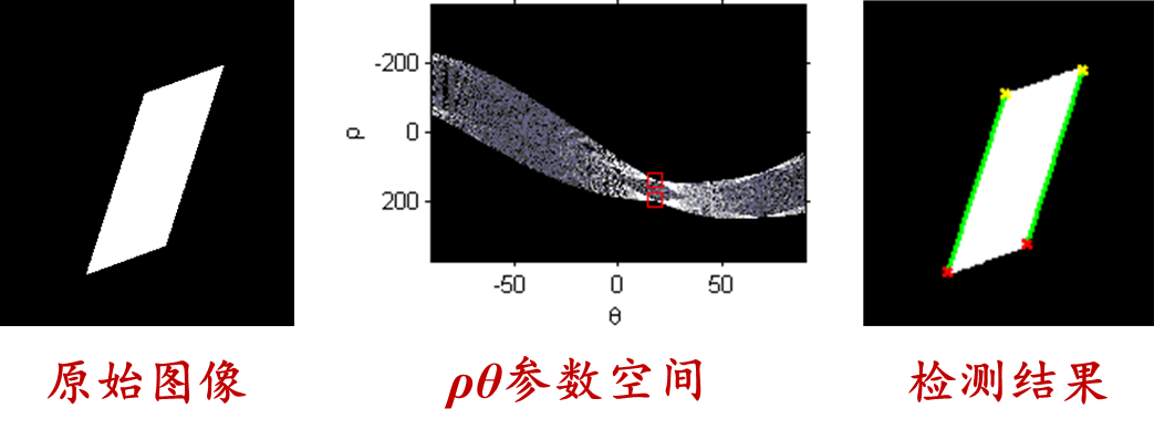
Hough transform : It is a technique widely used in the fields of image processing and computer vision. It was originally proposed by Hough in 1962 for detecting straight lines in images, but was later extended to detect other shapes such as circles, ellipses, etc. The Hough transform is mainly used to detect geometric shapes in images and has good robustness to noise and incomplete shape edges. The core idea is to establish a point-line dual relationship , transform the image from image space to parameter space, determine the parameters of the curve, and then determine the curve in the image. If the shape of the boundary line is known, the curve parameters are determined by detecting discrete boundary points in the image, and the boundary curve is redrawn in the image space, thereby improving the boundary. Proceed as follows

Edge detection : First, the image needs to be edge detected in order to process the edge points in the Hough transform. You can use methods such as Canny edge detection to get the edges of the image
Parameter space representation : For the geometric shape to be detected (such as a straight line), an appropriate parameter representation needs to be selected. For example, for a straight line, polar coordinates (ρ, θ) are usually used to represent it, where ρ represents the vertical distance from the origin to the straight line, and θ represents the inclination angle of the straight line.
Accumulator array : Create an accumulator array, initializing the count to 0 for every possible parameter combination (ρ, θ) in parameter space
Voting process : For each edge point in the edge image, vote on the accumulator array according to its possible parameters (ρ, θ) in the parameter space, that is, add one to the corresponding count value
Threshold setting : Based on the voting results in the accumulator array, a threshold can be set for determining the detected geometry. Only when the count value in the accumulator array is greater than the set threshold, it is considered a valid geometry
Parameter inverse transformation : According to the valid votes in the accumulator array, the parameters are inversely transformed back to the original image space to obtain the position of the detected geometric shape in the image.

The Hough transform is highly robust and widely used in detecting shapes such as straight lines, circles, ellipses, etc. in images. However, the computational complexity of Hough transform is high, and the detection of large-scale images or complex shapes may require more computing resources. Therefore, in practical applications, you can choose to use Hough transform or other more efficient methods to detect geometric shapes depending on the specific situation.

as follows

Insert image description here

matlab implementation :

Image=rgb2gray(imread('houghsource.bmp'));
bw=edge(Image,'canny');
figure,imshow(bw);
[h,t,r]=hough(bw,'RhoResolution',0.5,'ThetaResolution',0.5);
figure,imshow(imadjust(mat2gray(h)),'XData',t,'YData',r,'InitialMagnification','fit');
xlabel('\theta'),ylabel('\rho');
axis on,axis normal,hold on;
P=houghpeaks(h,2);
x=t(P(:,2));
y=r(P(:,1));
plot(x,y,'s','color','r');
lines=houghlines(bw,t,r,P,'FillGap',5,'Minlength',7);
figure,imshow(Image);
hold on;
max_len=0;
for i=1:length(lines)
    xy=[lines(i).point1;lines(i).point2];
    plot(xy(:,1),xy(:,2),'LineWidth',2,'Color','g');
    plot(xy(1,1),xy(1,2),'x','LineWidth',2,'Color','y');
    plot(xy(2,1),xy(2,2),'x','LineWidth',2,'Color','r');
end

python implementation :

import cv2
import numpy as np
import matplotlib.pyplot as plt

# 读取图像并转换为灰度图像
image = cv2.imread('houghsource.bmp')
image_gray = cv2.cvtColor(image, cv2.COLOR_BGR2GRAY)

# 边缘检测
bw = cv2.Canny(image_gray, 100, 200)

# 显示边缘图像
plt.figure()
plt.imshow(bw, cmap='gray')
plt.title('边缘图像')
plt.show()

# Hough变换
h, t, r = cv2.HoughLines(bw, rho=0.5, theta=np.pi/360, threshold=100)

# 显示Hough变换结果
plt.figure()
plt.imshow(np.log(1 + h), extent=[np.rad2deg(t[-1]), np.rad2deg(t[0]), r[-1], r[0]],
           cmap='gray', aspect=1/2)
plt.title('Hough变换结果')
plt.xlabel('Theta (degrees)')
plt.ylabel('Rho')
plt.show()

# 提取Hough变换的峰值点
P = cv2.HoughPeaks(h, 2, np.pi/360, threshold=100)

# 显示提取的峰值点
plt.figure()
plt.imshow(np.log(1 + h), extent=[np.rad2deg(t[-1]), np.rad2deg(t[0]), r[-1], r[0]],
           cmap='gray', aspect=1/2)
plt.title('Hough变换结果（峰值点）')
plt.xlabel('Theta (degrees)')
plt.ylabel('Rho')
plt.plot(np.rad2deg(t[P[:, 1]]), r[P[:, 0]], 's', color='r')
plt.show()

# 提取直线并在原图上绘制
lines = cv2.HoughLinesP(bw, 1, np.pi/180, threshold=100, minLineLength=7, maxLineGap=5)

plt.figure()
plt.imshow(cv2.cvtColor(image, cv2.COLOR_BGR2RGB))
plt.title('检测到的直线')
plt.xlabel('x')
plt.ylabel('y')
plt.xlim(0, image.shape[1])
plt.ylim(image.shape[0], 0)

for line in lines:
    x1, y1, x2, y2 = line[0]
    plt.plot([x1, x2], [y1, y2], 'g-', linewidth=2)
    plt.plot(x1, y1, 'yx', markersize=8)
    plt.plot(x2, y2, 'rx', markersize=8)

plt.show()

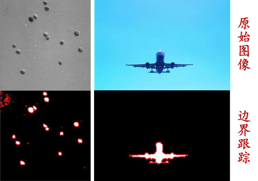
(3) Boundary tracking

Boundary tracking : is a technique used in image processing and computer vision to extract object contours. The goal of boundary tracking is to find the boundary pixels of the object in the image to obtain the contour information of the object. Boundary tracking algorithms usually start from a starting point and track along the boundary pixels of the object until returning to the starting point. The tracking process is based on the connectivity of pixels, finding the next adjacent boundary pixel from the current pixel, and then jumping to this pixel for tracking until returning to the starting point. The following are the basic steps of a simple boundary tracking algorithm (8-neighbor tracking algorithm)

Select starting point : Select a pixel in the image as the starting point, which should be located on the boundary of the object
8-neighborhood search : Starting from the starting point, search for adjacent pixels in an 8-neighborhood manner. For the current pixel, check its 8 neighboring pixels (top, bottom, left, right, top left, top right, bottom left, bottom right), find the first boundary pixel (usually a non-background pixel), and then update the current pixel to the boundary pixel and add the boundary pixel to the boundary point set
Continue tracking : Repeat step 2 until you return to the starting point
Stop tracking : When you return to the starting point, the boundary tracking ends. At this time, the pixels stored in the boundary point set are the outline information of the object.

Boundary tracking algorithms can be used for object detection, image segmentation, contour extraction and other applications. Different boundary tracking algorithms have different connectivity requirements and termination conditions. Common boundary tracking algorithms also include 4-neighbor tracking algorithm and Moore-Neighbor tracking algorithm. In practical applications, appropriate boundary tracking algorithms can be selected based on image characteristics and application requirements.

as follows

Insert image description here

matlab implementation :

Image=im2bw(imread('algae.jpg'));
Image=1-Image;                      %bwboundaries函数以白色区域为目标，本图中目标暗，因此反色。
[B,L]=bwboundaries(Image);
figure,imshow(L),title('划分的区域');
hold on;
for i=1:length(B)
    boundary=B{
    
    i};
    plot(boundary(:,2),boundary(:,1),'r','LineWidth',2);
end

python implementation :

import cv2
import numpy as np
import matplotlib.pyplot as plt

# 读取图像并转换为二值图像
image = cv2.imread('algae.jpg')
image_gray = cv2.cvtColor(image, cv2.COLOR_BGR2GRAY)
_, Image = cv2.threshold(image_gray, 128, 255, cv2.THRESH_BINARY)

# 反色处理
Image = 255 - Image

# 使用cv2.findContours函数获取边界点
contours, _ = cv2.findContours(Image, cv2.RETR_EXTERNAL, cv2.CHAIN_APPROX_SIMPLE)

# 绘制边界
plt.figure()
plt.imshow(Image, cmap='gray')
plt.title('划分的区域')
plt.xlabel('x')
plt.ylabel('y')

for contour in contours:
    contour = contour.squeeze()
    plt.plot(contour[:, 1], contour[:, 0], 'r', linewidth=2)

plt.show()