Article directory
1: Geometric description
(1) Geometric relationship between pixels
A: Adjacency and connectivity
Foreground and background :
- Foreground : Refers to a target or object of interest in an image , which usually has a higher pixel value (brightness or color) and is visually distinguished from other parts. At the pixel level, foreground pixels are usually clustered together to form a continuous area , representing the outer contour or internal information of the target.
- Background : refers to the image area outside the foreground . It usually contains the foreground and provides the environment and contextual information of the foreground. Background pixels typically have lower pixel values (brightness or color) and are visually distinct from foreground areas
In terms of geometric relationships, there are many relationships between the foreground and the background, such as:
- Foreground-background segmentation : This is an important task in image processing and computer vision, which is to segment the foreground objects in the image from the background. By analyzing features such as geometric relationships, pixel values, and texture of pixels, foreground-background segmentation can be performed to identify and extract target areas of interest.
- Foreground-background interaction : In an image, the foreground and background may interact or influence each other. For example, in portrait photography, the subject is usually the foreground, with the background providing a suitable context. Better visual effects can be achieved by adjusting the relationship between the foreground and background
- Foreground-background constraints : In the field of computer vision, the geometric relationship between the foreground and background can be used to constrain the results of analysis and processing. For example, in object recognition, the accuracy of target detection and classification can be improved by considering geometric features such as the boundary and proportional relationship between the foreground and background.
Paths and connections :
- Path : refers to a continuous line or curve from one pixel to another . In image processing and computer vision, paths are often used to describe the boundaries, contours, or connections between pixels of objects . Paths can be represented in different forms, such as pixel sequences in binary images, continuous edge points, polygons, etc.
- Contour path : In target segmentation and recognition, the contour path represents the shape boundary of the target and is formed by connecting pixels on the target boundary.
- Skeleton path : The skeleton path is also called the central axis, which represents the main structural or morphological characteristics of the target and is formed by connecting the pixels inside the target.
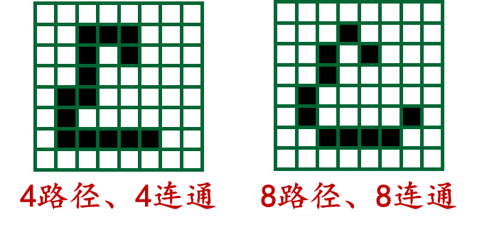
- Connectivity : refers to the direct adjacency relationship between pixels, that is, adjacent pixels are connected by sharing edges or corners . At the pixel level, connectivity can be defined in terms of four-neighborhood or eight-neighborhood. Four-neighborhood represents four adjacent pixels in the upper, lower, left, and right directions, and eight-neighborhood represents eight adjacent pixels in the upper, lower, left, right, and diagonal directions.
- 4-connected : In a four-neighborhood, if two pixels share an edge between them, they are considered 4-connected.
- 8-connected : In an eight-neighborhood, if two pixels share an edge or a corner, they are considered 8-connected.
B: distance
Distance : for pixels ppp、 q q q和 z z z , if the following three conditions are met, it is calledddd is the distance function or metric
- d ( p , q ) ≥ 0 d(p,q)\geq 0d(p,q)≥0
- d ( p , q ) = d ( q , p ) d(p,q)=d(q,p) d(p,q)=d(q,p)
- d ( p , z ) ≤ d ( p , q ) + d ( q , z ) d(p,z)\leq d(p,q)+d(q,z) d(p,z)≤d(p,q)+d(q,z)
Among them, the Euclidean distance refers to
D e ( p , q ) = ( x − s ) 2 + ( y − t ) 2 D_{e}(p, q)=\sqrt{(x-s)^{2}+(y-t)^{2}} De(p,q)=(x−s)2+(y−t)2
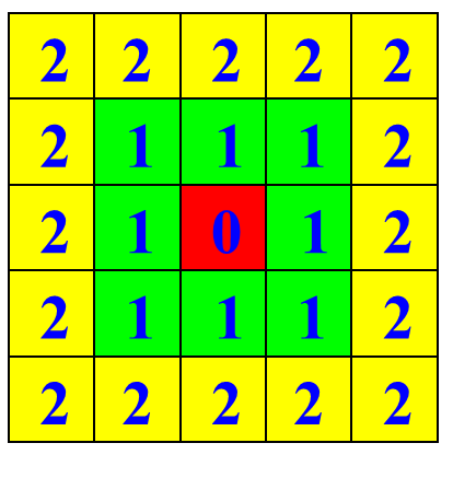
City distance : D 4 ( p , q ) = ∣ x − s ∣ + ∣ y − t ∣ D_{4}(p,q)=|xs|+|yt|D4(p,q)=∣x−s∣+∣y−t∣

Board distance : D 8 ( p , q ) = max ( ∣ x − s ∣ , ∣ y − t ∣ ) D_{8}(p,q)=max(|xs|,|yt|)D8(p,q)=max(∣x−s∣,∣y−t∣)
(2) Geometric features between pixels
A: location
Position : The position of the object in the image, represented by the center point of the object area. The binary image quality distribution is uniform, and the centroid and centroid coincide. If the pixel position coordinates corresponding to the object in the image are (xi, yi) (i = 0, 1, …, n - 1; j = 0, 1, …, m - 1) (x_{i},y_{i })(i=0, 1, …, n-1; j=0, 1, …, m-1)(xi,yi)(i=0,1,…,n -1 ;j=0,1,…,m - 1 ) , then the coordinates of the center of mass position are
x ˉ = 1 m n ∑ i = 0 n − 1 ∑ j = 0 m − 1 x i ; y ˉ = 1 m n ∑ i = 0 n − 1 ∑ j = 0 m − 1 y j \bar{x}=\frac{1}{m n} \sum_{i=0}^{n-1} \sum_{j=0}^{m-1} x_{i} ; \bar{y}=\frac{1}{m n} \sum_{i=0}^{n-1} \sum_{j=0}^{m-1} y_{j} xˉ=mn1i=0∑n−1j=0∑m−1xi;yˉ=mn1i=0∑n−1j=0∑m−1yj
B: direction
Direction : If the object is elongated, the axis of the longer direction can be defined as the direction of the object. Define the minimum second-order moment axis (the equivalent axis of the minimum inertia axis on a two-dimensional plane) as the direction of the longer object. In other words, we need to find a straight line such that EE defined by the following formulaE value is the smallest
E = ∬ r 2 f ( x , y ) d x d y E=\iint r^{2} f(x, y) d x d y E=∬r2f(x,y)dxdy
C: size
Length and width : When the boundary of an object is known, using the size of its circumscribed rectangle to describe its basic shape is the simplest way to find the circumscribed rectangle of the object in the direction of the coordinate system. You only need to calculate the maximum and minimum coordinates of the object's boundary points. value, you can get the horizontal and vertical span of the object
- Minimum circumscribed rectangle : For objects in any orientation, horizontal and vertical are not the directions we are interested in. It is necessary to determine the main axis of the object, and then calculate the length in the direction of the main axis and the width in the direction perpendicular to it that reflect the shape characteristics of the object. Such a circumscribed rectangle is the object's main axis.
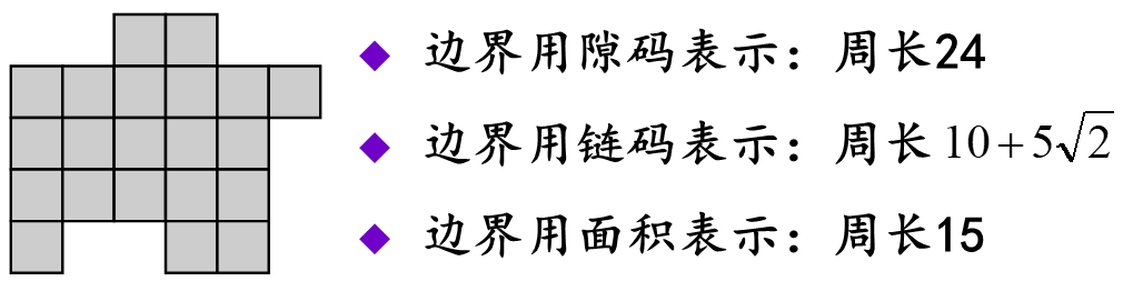
Perimeter : The boundary length of a region, used to distinguish objects with simple or complex shapes; different representation methods lead to different calculation methods
- The boundary is represented by a gap code : if the pixels in the image are regarded as small squares per unit area, then the area and background in the image are composed of small squares. The perimeter of the area is the sum of the lengths of the area and the background gap, and the boundary is represented by a gap code. Therefore, finding the perimeter is to calculate the length of the gap code
- The boundary is represented by a chain code : when pixels are regarded as points, the perimeter is represented by a chain code. To find the perimeter is to calculate the length of the chain code.
- The boundary is expressed by area : that is, the sum of the number of boundary points, each point occupies a small square with an area of 1
Area : measures the total size of an object, which is only related to the boundary of the object and has nothing to do with changes in its internal gray level. The pixel count area is
- Count the number of pixels inside the boundary (also on the boundary)
- For a binary image, if 1 is used to represent the object and 0 is used to represent the background, its area is the statistics f (x, y) = 1 f(x,y)=1f(x,y)=number of 1
(3) Procedure
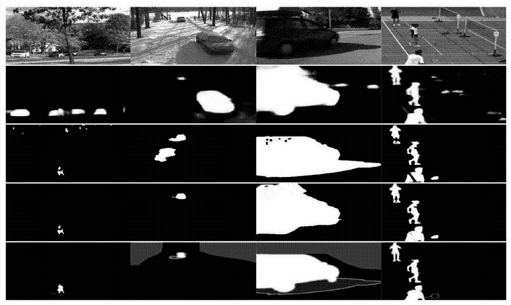
As follows: perform threshold segmentation on the image and count the geometric features of the area
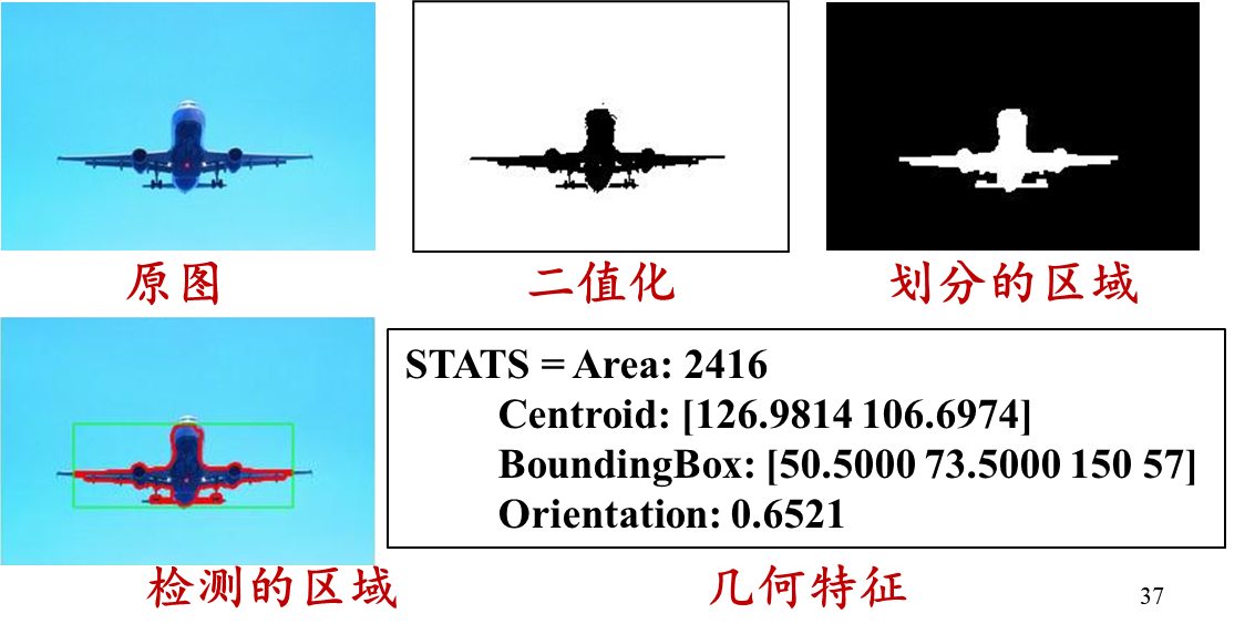
matlab:
clear,clc,close all;
image=imread('plane.jpg');
BW=im2bw(rgb2gray(image));
figure,imshow(BW),title('二值化图像');
% imwrite(BW,'biplane.jpg');
SE=strel('square',3);
Morph=imopen(BW,SE);
Morph=imclose(Morph,SE);
figure,imshow(Morph),title('形态学滤波');
% imwrite(Morph,'morphplane.jpg');
[B,L]=bwboundaries(1-Morph);
figure,imshow(L),title('划分的区域');
% imwrite(L,'Lplane.jpg');
STATS = regionprops(L,'Area', 'Centroid','Orientation','BoundingBox');
figure,imshow(image),title('检测的区域');
hold on;
for i=1:length(B)
    boundary=B{

    i};
    plot(boundary(:,2),boundary(:,1),'r','LineWidth',2);
end
rectangle('Position',STATS.BoundingBox,'edgecolor','g');
hold off;
% STATS
python:
import numpy as np
import cv2
import matplotlib.pyplot as plt

image = cv2.imread('plane.jpg')
gray = cv2.cvtColor(image, cv2.COLOR_BGR2GRAY)
_, bw = cv2.threshold(gray, 127, 255, cv2.THRESH_BINARY)
plt.imshow(bw, cmap='gray')
plt.title('二值化图像')
plt.show()

kernel = cv2.getStructuringElement(cv2.MORPH_RECT, (3, 3))
morph = cv2.morphologyEx(bw, cv2.MORPH_OPEN, kernel)
morph = cv2.morphologyEx(morph, cv2.MORPH_CLOSE, kernel)
plt.imshow(morph, cmap='gray')
plt.title('形态学滤波')
plt.show()

contours, _ = cv2.findContours(255 - morph, cv2.RETR_EXTERNAL, cv2.CHAIN_APPROX_SIMPLE)
boundary_image = np.zeros_like(morph)
cv2.drawContours(boundary_image, contours, -1, 255, 1)
plt.imshow(boundary_image, cmap='gray')
plt.title('划分的区域')
plt.show()

stats = []
for contour in contours:
    area = cv2.contourArea(contour)
    centroid = np.mean(contour, axis=0)[0]
    rect = cv2.boundingRect(contour)
    stats.append({


        'Area': area,
        'Centroid': centroid,
        'BoundingBox': rect
    })

image_with_boundary = image.copy()
for boundary in contours:
    cv2.drawContours(image_with_boundary, [boundary], -1, (0, 0, 255), 2)

for stat in stats:
    cv2.rectangle(image_with_boundary, stat['BoundingBox'], (0, 255, 0), 2)

plt.imshow(cv2.cvtColor(image_with_boundary, cv2.COLOR_BGR2RGB))
plt.title('检测的区域')
plt.show()
2: Shape description
(1) Rectangularity
Rectangularity : A quantitative indicator used to describe how close an entity or area is to a rectangle. It measures how similar an object or area is to a rectangle in shape, that is, its compactness and regularity . Rectangularity is calculated by comparing the object's actual area to the area of the smallest bounding rectangle (Bounding Rectangle) . The smallest enclosing rectangle is the smallest area rectangle that can completely surround the object. Its length and width are consistent with the main direction of the object. The calculation formula for rectangularity is as follows
- A o A_{o}Ao:The area of the object
- A M E R A_{MER} AMER: Area of MER
R = A o A M E R R=\frac{A_{o}}{A_{MER}} R=AMERAo
The ratio of MER width to length is
r = W M E R L M E R r=\frac{W_{MER}}{L_{MER}} r=LMERWMER
(2) Circularity
A: roundness
Roundness : A quantitative indicator used to describe the closeness of an entity or area to a circle . It measures how similar an object or area is to a circle in shape, its circularity. Roundness is calculated by comparing the object's actual area to the area of an equivalent circle. An equivalent circle is a circle with the same area as the object, whose radius can be calculated by dividing the object's area by π and then taking the square root. The formula for calculating roundness is as follows
- F = 1 F=1 F=1 : The area is a circle
- F < 1 F<1 F<1 : The area is in other shapes
- The more complex the region boundary curvature is, the more the region's characteristics deviate from the circle, the smaller F will be
F = 4 π AP 2 F=\frac{4\pi A}{P^{2}}F=P24 p A
B: Boundary energy
Boundary energy : curvature function of points on the boundary
- P P P : Perimeter of the object
- p p p : The distance from the point on the boundary to a starting point
- r ( p ) r(p) r ( p ) : instantaneous radius of curvature at a point on the boundary. is the radius of the tangent circle between the point and the boundary
- K ( p ) K(p) K ( p ) : is a periodic function with period P
K ( p ) = 1 r ( p ) K(p)=\frac{1}{r(p)} K(p)=r(p)1

C: circularity
Circularity : is a metric used to describe the shape of a solid or object as close to a sphere . It measures how similar an object or area is to a sphere in shape. Circularity is calculated by comparing the object's volume to the volume of an equivalent sphere. An equivalent sphere is a sphere with the same volume as the object, its radius can be calculated by dividing the object's volume by (4/3π) and then taking the cube root
C = μ R σ R 2 μ R = 1 K ∑ k = 0 K − 1 ∥ ( xk , yk ) − ( x ˉ , y ˉ ) ∥ σ R 2 = 1 K ∑ k = 0 K − 1 [ ∥ ( xk , yk ) − ( x ˉ , y ˉ ) ∥ − μ R ] 2 \begin{array}{l}C=\frac{\mu_{R}}{\sigma_{R}^{2}} \\ \mu_{R}=\frac{1}{K} \sum_{k=0}^{K-1}\left\|\left(x_{k}, y_{k}\right)-(\bar {x}, \bar{y})\right\| \\\sigma_{R}^{2}=\frac{1}{K}\sum_{k=0}^{K-1}\left[\left\|\left(x_{k}, y_{ k}\right)-(\bar{x}, \bar{y})\right\|-\mu_{R}\right]^{2}\end{array}C=pR2mRmR=K1∑k=0K−1∥(xk,yk)−(xˉ,yˉ)∥pR2=K1∑k=0K−1[∥(xk,yk)−(xˉ,yˉ)∥−mR]2
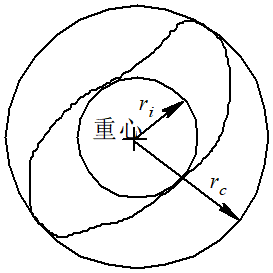
D: Radius ratio of inscribed circle and circumscribed circle
The ratio of the radius of the inscribed circle to the circumscribed circle : the complexity of describing the boundary of an object
- r i r_{i} ri: Radius of the inscribed circle of the area
- r c r_{c} rc: Area circumscribed circle radius
S = r i r c S=\frac{r_{i}}{r_{c}} S=rcri
The centers of both circles are at the center of gravity of the region
- When the area is a circle, SSSmax 1.0
- For other shapes, there is SSS<1.0
- S S S is not affected by regional translation, rotation and scale changes
E: program
As follows, segment the original image and detect circles and rectangles
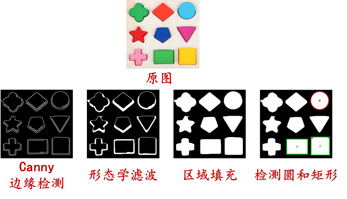
matlab:
clear,clc,close all;
image=rgb2gray(imread('shape.png'));
figure,imshow(image),title('Ôͼ');
BW=edge(image,'canny');
figure,imshow(BW),title('±ß½çͼÏñ');
% imwrite(BW,'shapeedge.jpg');
SE=strel('disk',5);
Morph=imclose(BW,SE);
figure,imshow(Morph),title('ÐÎ̬ѧÂ˲¨');
% imwrite(Morph,'shapemorph.jpg');
Morph=imfill(Morph,'holes');
figure,imshow(Morph),title('ÇøÓòÌî³ä');
imwrite(Morph,'shapefill.jpg');
[B,L]=bwboundaries(Morph);
figure,imshow(L),title('¼ì²âÔ²ºÍ¾ØÐÎ');
% imwrite(L,'Lplane.jpg');
STATS = regionprops(L,'Area', 'Centroid','BoundingBox');
len=length(STATS);
hold on
for i=1:len
R=STATS(i).Area/(STATS(i).BoundingBox(3)*STATS(i).BoundingBox(4));
boundary=fliplr(B{
i});
everylen=length(boundary);
F=4*pi*STATS(i).Area/(everylen^2);
dis=pdist2(STATS(i).Centroid,boundary,'euclidean');
miu=sum(dis)/everylen;
sigma=sum((dis-miu).^2)/everylen;
C=miu/sigma;
if R>0.9 && F<1
rectangle('Position',STATS(i).BoundingBox,'edgecolor','g','linewidth',2);
plot(STATS(i).Centroid(1),STATS(i).Centroid(2),'g*');
end
if R>pi/4-0.1 && R<pi/4+0.1 && F>0.9 && C>10
rectangle('Position',[STATS(i).Centroid(1)-miu,STATS(i).Centroid(2)-miu,2*miu,2*miu],...
'Curvature',[1,1],'edgecolor','r','linewidth',2);
plot(STATS(i).Centroid(1),STATS(i).Centroid(2),'r*');
end
end
hold off
python:
import cv2
import numpy as np
import matplotlib.pyplot as plt

# 读取图像并将其转换为灰度图像
image = cv2.imread('shape.png')
gray = cv2.cvtColor(image, cv2.COLOR_BGR2GRAY)

# 显示原始图片
plt.imshow(cv2.cvtColor(image, cv2.COLOR_BGR2RGB))
plt.title('原始图像')
plt.show()

# 边缘检测
edges = cv2.Canny(gray, 30, 100)

# 显示边缘图片
plt.imshow(edges, cmap='gray')
plt.title('边缘图像')
plt.show()

# 闭运算
kernel = cv2.getStructuringElement(cv2.MORPH_ELLIPSE, (5, 5))
closed = cv2.morphologyEx(edges, cv2.MORPH_CLOSE, kernel)

# 显示闭运算结果
plt.imshow(closed, cmap='gray')
plt.title('闭运算')
plt.show()

# 填充内部空洞
filled = cv2.fillHoles(closed)

# 显示填充结果
plt.imshow(filled, cmap='gray')
plt.title('填充后图像')
plt.show()

# 寻找轮廓并进行形状分析
contours, _ = cv2.findContours(filled, cv2.RETR_EXTERNAL, cv2.CHAIN_APPROX_SIMPLE)
for cnt in contours:
    area = cv2.contourArea(cnt)
    x, y, w, h = cv2.boundingRect(cnt)
    rect_ratio = area / (w * h)
    perimeter = cv2.arcLength(cnt, True)
    circularity = 4 * np.pi * area / (perimeter ** 2)
    centroid = (int(x + w / 2), int(y + h / 2))
    distance = cv2.pointPolygonTest(cnt, centroid, True)

    if rect_ratio > 0.9 and circularity < 1:
        cv2.rectangle(image, (x, y), (x + w, y + h), (0, 255, 0), 2)
        cv2.circle(image, centroid, 3, (0, 255, 0), -1)

    if np.abs(circularity - np.pi / 4) < 0.1 and rect_ratio > 0.9 and distance > 10:
        cv2.rectangle(image, (int(centroid[0] - distance), int(centroid[1] - distance)),
                      (int(centroid[0] + distance), int(centroid[1] + distance)), (0, 0, 255), 2)
        cv2.circle(image, centroid, 3, (0, 0, 255), -1)

# 显示最终结果
plt.imshow(cv2.cvtColor(image, cv2.COLOR_BGR2RGB))
plt.title('形状分析结果')
plt.show()
(3) Central axis transformation
A: concept
Medial axis transformation : It is an image processing technology used to extract the central axis features of an object or region . The central axis is a curve that is tangent to the object boundary and has the largest inscribed circle. The basic idea of the central axis transformation is to gradually shrink inward on the boundary of the object through iterative operations until it reaches the position of the central axis . In this process, the distance from each boundary point to the nearest inscribed circle is calculated, and these distance values are added together to form a distance field. Through threshold processing and connection operations, the central axis can be obtained. The basic steps are as follows
- Preprocess the image , such as grayscale, binarization and other operations to separate the object from the background.
- To find the boundaries of an object , you can use an edge detection algorithm (such as Canny edge detection) to get the edges of a binary image
- Initialize an empty image as a distance field with the same size as the original image
- Starting from the boundary points of the object, do the following for each boundary point
- Calculate the radius of the nearest inscribed circle from the current boundary point to the interior of the object
- Store the radius value at the corresponding location in the distance field
- According to the threshold of the distance field, it is binarized to obtain the central axis image.
- Perform connection operations and process the central axis image to make the central axis continuous and uninterrupted

Medial axis transformation is commonly used in fields such as shape analysis, morphological processing, and feature extraction. By extracting the central axis of an object, the structural information and geometric characteristics of the object can be obtained, which is helpful for applications such as shape analysis, target recognition, and image reconstruction. It should be noted that the results of medial axis transformation are affected by factors such as image preprocessing, threshold selection, and connection methods. Therefore, in practical applications, parameter adjustment and optimization may need to be performed according to specific conditions to obtain better central axis results.
B:Program
As follows, extract the target image skeleton
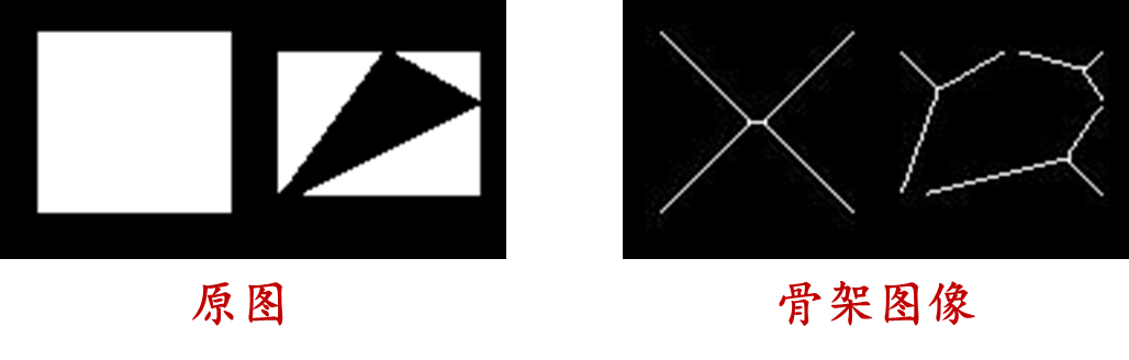
matlab:
clear,clc,close all;
Image=imread('test.bmp');
BW=im2bw(Image);
figure,imshow(BW);
result=bwmorph(BW,'skel',Inf);
figure,imshow(result);
python:
import cv2
import numpy as np
import matplotlib.pyplot as plt

# 读取图像并转换为二值图像
image = cv2.imread('test.bmp', 0)
ret, bw = cv2.threshold(image, 127, 255, cv2.THRESH_BINARY)

# 显示原始二值图像
plt.imshow(bw, cmap='gray')
plt.title('原始二值图像')
plt.show()

# 中轴变换
skeleton = np.zeros_like(bw)
size = np.size(bw)
element = cv2.getStructuringElement(cv2.MORPH_CROSS, (3,3))

while True:
    eroded = cv2.erode(bw, element)
    temp = cv2.dilate(eroded, element)
    temp = cv2.subtract(bw, temp)
    skeleton = cv2.bitwise_or(skeleton, temp)
    bw = eroded.copy()

    zeros = size - cv2.countNonZero(bw)
    if zeros == size:
        break

# 显示中轴图像
plt.imshow(skeleton, cmap='gray')
plt.title('中轴图像')
plt.show()