Data analysis - user consumption behavior analysis

---

Preface

User behavior runs through all walks of life. By analyzing user consumption behavior, it can help companies better understand their development status, make timely strategic adjustments, and make the company run better. This article uses the details of the number of CDs purchased by users of an e-commerce website as sample data to sort out the specific content of analyzing user consumption behavior.

---

1. Data preprocessing

The data analyzed in this article is text type data without column names. In order to facilitate subsequent analysis, it is necessary to add column headers to this data. The code is as follows:

columns=['user_id','order_dt','order_products','order_amount']
df=pd.read_table('CDNOW_master.txt',names=columns,sep='\s+')

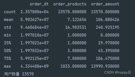
The specific information of the data is as follows:

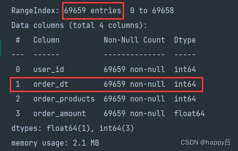
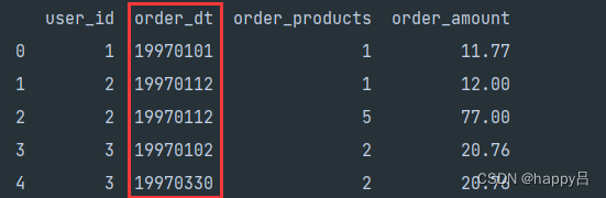
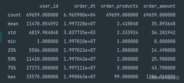
Observing the data, we can find that: ① The data volume is large, but the data is complete and there are no missing values; ② The date is of int type and needs to be formatted; ③ The same user purchases multiple times in one day; ④ The average user Each order purchases 2~3 products, with a standard deviation of 2.3 and little fluctuation. The value at the 75% quantile of the user's purchase quantity is 3, indicating that the purchase volume of most orders is not large; ⑤ The purchase amount reflects Most of the order consumption amounts are concentrated in small and medium amounts, with an average of around 35.

Based on the conclusions drawn from the above observations, the following adjustments are made to the data date:
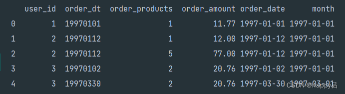
First, convert the date format and put it into the 'order_date' column. The code is as follows:

df['order_date']=pd.to_datetime(df['order_dt'],format='%Y%m%d')

In order to facilitate the subsequent analysis of data by month, a new column "month" is added to store the date with a precision of month. The code is as follows:

df['month']=df['order_date'].values.astype('datetime64[M]')

The modified data is as follows:

---

2. Analysis of overall consumption trends of users (by month)

Statistics of product purchase quantity, consumption amount, consumption times, and number of consumers are calculated by month. The specific codes are as follows:

plt.figure(figsize=(20,15)) # 单位是英寸
plt.subplot(221) # 绘子图 两行两列，占据第一个位置
# 每月的购买数量
df.groupby(by='month')['order_products'].sum().plot() # 默认折线图
plt.title('每月的购买数量')
# 每月的消费金额
plt.subplot(222)
df.groupby(by='month')['order_amount'].sum().plot()
plt.title('每月的消费金额')
# 每月的消费次数
plt.subplot(223)
df.groupby(by='month')['user_id'].count().plot()
plt.title('每月的消费次数')
# 每月的消费人数
plt.subplot(224)
df.groupby(by='month')['user_id'].apply(lambda x:len(x.drop_duplicates())).plot()
plt.title('每月的消费人数')
plt.show()

Analysis:
① It can be seen from Figure 1, Figure 2 and Figure 3 that the number of goods purchased by users each month, the amount of consumption, and the number of times each user enters the store to make purchases, all showed an upward trend from January to March. ~A sharp decline in April, then fluctuating to a plateau.
② The number of people entering the store each month showed an upward trend from January to February, and then dropped sharply to a stable state. Specifically, the number of consumers in the first three months was around 8,000 to 10,000, and the average number of consumers in the subsequent months was around 2,000.
③ Reason analysis: January, February, and March are around the Spring Festival, and consumer demand increases; the company may increase promotional efforts in January, February, and March, which will increase the sales quantity, amount, and number of user purchases of goods in the first three months. rise. However, the number of consumers has begun to decline since February. It is speculated that the product may have a better experience, converting some new customers into regular customers.

---

3. User’s individual consumption analysis

1 Descriptive statistics of user consumption amount and consumption times (number of products)

user_grouped=df.groupby(by='user_id').sum()
print(user_grouped.describe())

Conclusion:
① User perspective: There are 23,570 users. Each user purchases an average of 7 products, but the median is 3, and the maximum purchase quantity is 1,033. The average is greater than the median, which is a typical right-skewed distribution. ② Consumption amount
perspective : The average user consumption is 106, the median is 43, and there are wealthy users who consume 13,990. Combining the quantile and the maximum value, the average is almost equal to the 75% quantile, which belongs to a right-skewed distribution. The picture above shows the products purchased by each user

. Scatter plot of quantity and consumption amount. From the figure, it can be seen that the user's consumption amount and purchase quantity show a linear trend. The average price of each product is about 15, and the extreme points of orders are relatively few (consumption amount>1000, or purchase quantity >60), the impact on the sample is not significant and can be ignored

2 Analysis of user consumption distribution

plt.figure(figsize=(12,4))
plt.subplot(121)
plt.xlabel('每个订单的消费金额') # y轴为某个消费金额出现的次数
df['order_amount'].plot(kind='hist',bins=50) # bins：区间划分的次数，影响柱子的宽度
plt.subplot(122)
plt.xlabel('每个用户购买产品的数量')
df.groupby(by='user_id')['order_products'].sum().plot(kind='hist',bins=50)
plt.show()

Conclusion: It can be seen from the figure that orders with a consumption amount of less than 100 account for the vast majority, and the user's purchase quantity is small, concentrated within 50. In general, users with low consumption amounts and purchase quantities of less than 50 account for the majority

3 Analysis of the proportion of users’ cumulative consumption amount (user’s contribution)

# 每个用户的消费金额
user_cumsum=df.groupby(by='user_id')['order_amount'].sum().sort_values().reset_index()
# 每个用户消费金额累加
user_cumsum['amount_cumsum']=user_cumsum['order_amount'].cumsum()
amount_cumsum=user_cumsum['amount_cumsum'].max()
# 前xx名用户的累计贡献率
# user_cumsum['prop']=user_cumsum['amount_cumsum']/amount_cumsum # 方法一
# user_cumsum['prop']=user_cumsum['amount_cumsum'].apply(lambda x:x/amount_cumsum) # 方法二
user_cumsum['prop']=user_cumsum.apply(lambda x:x['amount_cumsum']/amount_cumsum,axis=1) # 方法三
print(user_cumsum.tail()) # 取最后5行
user_cumsum['prop'].plot()
plt.savefig('figs/savefig4.png')
plt.show()

Conclusion: The first 20,000 users contributed 40% of the total amount, and the remaining 3,500 users contributed 60% (2/8 principle)

4. Analysis of user consumption behavior

1 Analysis of first purchase time

df.groupby(by='user_id')['order_date'].min().value_counts().plot()
plt.savefig('figs/savefig5.png')
plt.show()

Conclusion: It can be seen from the figure that the first time users buy CDs is concentrated before April. It is speculated that the company increased its promotional efforts from January to April and attracted many new users. Overall, new customers showed an upward trend before February, and then showed a downward trend after February. It is speculated that this is due to the company's promotion efforts or price adjustments.

2 Analysis of last purchase time

df.groupby(by='user_id')['order_date'].max().value_counts().plot()
plt.savefig('figs/savefig5.png')
plt.show()

Conclusion: The last purchase time of most users was concentrated in the first three months, and there were few loyal users; the number of users who purchased the last product dropped sharply in mid-March, but as time went by, the number of users who purchased the last product increased again. trend. It is speculated that this data selects the tracking records of consumer users in the first 3 months in the following 18 months.

3 User stratification

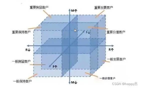
Build an RFM model : R represents the latest purchase date, F represents the number of purchases (frequency), and M is the purchase amount

# 构建数据透视表
rfm=df.pivot_table(index='user_id',
                   values=['order_products','order_amount','order_date'],
                   aggfunc={
    
    
                       'order_date':'max',
                       'order_products':'sum',
                       'order_amount':'sum'
                   })
rfm['R']=(rfm['order_date'].max()-rfm['order_date'])/np.timedelta64(1,'D') # 取相差的天数，保留一位小数，值越小越好
rfm.rename(columns={
    
    'order_amount':'M','order_products':'F'},inplace=True)

# RFM计算方式：每一列数据减去数据所在列的平均值，有正有负，与1作比较，大于置为1，小于1置为0
def rfm_func(x):
    level=x.apply(lambda x:'1' if x>=1 else '0')
    label=level['R']+level['F']+level['M']
    d={
    
    
        '111':'重要价值客户',
        '011':'重要保持客户',
        '101':'重要发展客户',
        '001':'重要挽留客户',
        '110':'一般价值客户',
        '010':'一般保持客户',
        '100':'一般发展客户',
        '000':'一般挽留客户',
    }
    result=d[label]
    return result

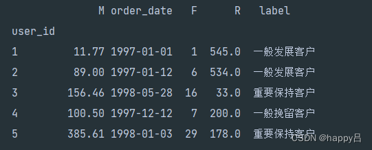
rfm['label']=rfm[['R','F','M']].apply(lambda x:x-x.mean()).apply(rfm_func,axis=1)
print(rfm.head())

Through the RFM model, customers are divided into: important value customers, important retention customers, important development customers, important retention customers, general value customers, general retention customers, general development customers, and general retention customers.


User hierarchical visualization

for label,grouped in rfm.groupby('label'):
    x=grouped['R']
    y=grouped['F']
    plt.scatter(x,y,label=label)
plt.legend() # 显示图例
plt.xlabel('R')
plt.ylabel('F')
plt.savefig('figs/savefig7.png')
plt.show()

rfm.groupby('label').size().plot()
plt.xticks(rotation=45)
plt.tight_layout() # 防止X轴标签显示不全

Conclusion: General users account for the vast majority, and there are only 4,000 important retained users out of 23,570 users. Some strategies should be formulated to improve the conversion rate of general users into important users.

4 Analysis of new customers, active users, and returning users

Definition:
Define customers who consume for the first time as new users.
Active users are old customers who have made purchases within a certain time window.
Inactive users are old customers who have not made purchases within the time window.
Returning users: equivalent to repeat customers. , can be divided into autonomous return flow and manual return flow. Autonomous return flow means that the customer returns by himself, while manual return flow is caused by human participation.

Processing data: Divide users into: new users, active users, inactive users, returning users and unconsumed users

pivoted_counts=df.pivot_table(index='user_id',
                              columns='month',
                              values='order_dt',
                              aggfunc='count').fillna(0) # 将nan填充为0

# 由于浮点数不直观，将其转换成是否消费，用 0、1表示
df_purchase=pivoted_counts.applymap(lambda x:1 if x>0 else 0)

# 判断是否是新用户、活跃用户、不活跃用户、回流用户
def active_status(data):
    status=[]
    for i in range(18): # 共有18列，即18个月
        if data[i]==0:
            if len(status)==0:
                status.append('unreg')
            else:
                if status[i - 1] == 'unreg':
                    status.append('unreg')
                else:
                    status.append('unactive')
        else:
            if len(status) == 0:
                status.append('new')
            else:
                if status[i - 1] == 'unactive':
                    status.append('return')
                elif status[i - 1] == 'unreg':
                    status.append('new')
                else:
                    status.append('active')
    return pd.Series(status,df_purchase.columns)

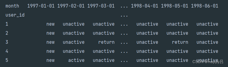
purchase_status=df_purchase.apply(active_status,axis=1)
print(purchase_status.head())

Analyze the number of users of each type

# 用nan代替unreg
purchase_status_ct=purchase_status.replace('unreg',np.NaN).apply(lambda x:pd.value_counts(x))
purchase_status_ct.T.fillna(0).plot.area()
plt.savefig('figs/savefig8.png')
plt.show()

Conclusion: In the first three months, red active users and blue new users accounted for a large proportion; after April, new users and active users began to decline, and showed a stable trend; returning users mainly appeared after April, and showed a stable trend. Is an important customer of the product.

Analysis of returning users and active users

rate=purchase_status_ct.T.fillna(0).apply(lambda x:x/x.sum(),axis=1)
# 回流用户占比
plt.plot(rate['return'],label='return')
# 活跃用户占比
plt.plot(rate['active'],label='active')
plt.legend()
plt.savefig('figs/savefig9.png')
plt.show()

Conclusion:
① Returning users: In the first six months, returning users increased, and then showed a downward trend, maintaining an average of 5%.
② Active users: Active users increased significantly in the first four months. It is speculated that the activity attracted many new users. In April After that, it began to decline and remained at about 2.5% on average.
③ After the website operation stabilized, the proportion of returning users was greater than that of active users.

5 User purchase cycle

order_diff=df.groupby(by='user_id').apply(lambda x:x['order_date']-x['order_date'].shift()) # 当前订单日期-上一次订单日期
print(order_diff.head())
print(order_diff.describe())
(order_diff/np.timedelta64(1,'D')).hist(bins=20)
plt.savefig('figs/savefig10.png')
plt.show()

Conclusion: As can be seen from the figure, the average consumption cycle is 68 days, and the consumption cycle of most users is less than 100 days, showing a typical long-tail distribution. Only a small number of users have a consumption cycle of more than 200 days (users who are not actively consuming)

Suggestion: For users who are not actively consuming, you can conduct a follow-up phone call about 3 days after their consumption, and increase the frequency of consumption through activities such as giving away coupons.

6 User life cycle

Calculation method: the user’s last purchase date - the first purchase date. If the difference = 0, it means the user only purchased once

user_life=df.groupby(by='user_id')['order_date'].agg(['min','max'])
(user_life['max']==user_life['min']).value_counts().plot.pie(autopct='%1.1f%%') # 格式化成1位小数
plt.legend(['仅消费一次','多次消费'])
plt.savefig('figs/savefig11.png')
plt.show()

Conclusion: More than half of the users only made a purchase once, indicating poor operation and poor retention rate.

print((user_life['max']-user_life['min']).describe()) # 生命周期分析

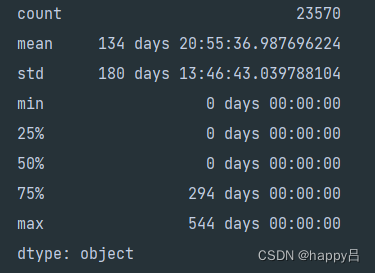
Conclusion: The average user life cycle is 134 days, but the median = 0, which once again verifies that most users consume once, and there are many low-quality users. Users after the 75% quantile have a life cycle greater than 294 days and are core users who need to focus on maintenance.

Draw a histogram of all user life cycles + multiple consumption

plt.figure(figsize=(12,6))
plt.subplot(121)
((user_life['max']-user_life['min'])/np.timedelta64(1,'D')).hist(bins=15)
plt.title('所有用户生命周期')
plt.xlabel('生命周期天数')
plt.ylabel('用户量')
plt.subplot(122)
u_l = (user_life['max']-user_life['min']).reset_index()[0]/np.timedelta64(1,'D')
u_l[u_l>0].hist(bins=15)
plt.title('多次消费用户生命周期')
plt.xlabel('生命周期天数')
plt.ylabel('用户量')
plt.savefig('figs/savefig12.png')
plt.show()

Conclusion:
① Comparison shows that the second picture filters out users with life cycle = 0, showing a bimodal structure.
② In Figure 2, there are also some users whose life cycle tends to 0. Although they have made multiple purchases, they cannot consume for a long time. They are ordinary users and can carry out targeted marketing and promotion activities.
③ A small number of users have a life cycle of 300 to 500 days, and they are loyal customers. Such users need to be vigorously maintained.

7 User repurchase rate and repurchase rate

Calculation method of repurchase rate: the proportion of users who have purchased multiple times among the total number of consumers in a natural month

# 自然月内复购用户用1表示，非复购用户用0表示，没有消费记录的用户用Nan表示
purchase_r=pivoted_counts.applymap(lambda x:1 if x>1 else np.NaN if x==0 else 0)
# nan数值不参与count计数
(purchase_r.sum()/purchase_r.count()).plot(figsize=(12,6)) # purchase_r.sum():复购用户人数  purchase_r.count()：总的消费人数
plt.savefig('figs/savefig13.png')
plt.show()

Conclusion: The repurchase rate began to increase in the first three months, and then stabilized and remained between 20% and 22%. The low repurchase rate in the first three months may be due to the large number of new users who only purchased once.

Repurchase rate calculation method : consumption is made within one time window, and consumption is made again within the next window

# 由于浮点数不直观，将其转换成是否消费，用 0、1表示
df_purchase=pivoted_counts.applymap(lambda x:1 if x>0 else 0)
def purchase_back(data):
    status=[]
    for i in range(17):
        if data[i]==1: # 当前月份消费了
            if data[i+1]==1:
                status.append(1) # 回购用户
            else:
                status.append(0)
        else: # 当前月份没有消费
            status.append(np.NaN)
    status.append(np.NaN) # 填充最后一列数据
    return pd.Series(status,df_purchase.columns)

purchase_b=df_purchase.apply(purchase_back,axis=1)

# 回购率可视化
plt.figure(figsize=(20,4))
plt.subplot(211)
# 回购率,nan不参与count计算
(purchase_b.sum()/purchase_b.count()).plot(label='回购率')
# 复购率
purchase_r=pivoted_counts.applymap(lambda x:1 if x>1 else np.NaN if x==0 else 0)
(purchase_r.sum()/purchase_r.count()).plot(label='复购率')
plt.ylabel('百分比%')
plt.title('用户回购率和复购率对比图')

# 回购人数与购物总人数
plt.subplot(212)
plt.plot(purchase_b.sum(),label='回购人数')
plt.plot(purchase_b.count(),label='购物总人数')
plt.title('回购人数与购物总人数')
plt.ylabel('人数')
plt.xlabel('month')
plt.legend()
plt.savefig('figs/savefig15.png')
plt.show()

Conclusion:
① It can be seen from the repurchase rate that it is around 30% after stabilization, with slightly higher volatility
② The repurchase rate is lower than the repurchase rate, and it is around 20% after stabilization and the volatility is small
③ Regardless of the repurchase rate in the first three months Both purchases and repurchases are showing an upward trend, indicating that it takes a certain amount of time for new users to become repurchase or repurchase users④
Combined with the analysis of new and old customers, the loyalty of new customers is much lower than the loyalty of old customers⑤
Total shopping in the first three months The number of people was far greater than the number of repurchases. Three months later, the number of repurchases and the total number of purchases began to stabilize. The number of repurchases stabilized at around 1,000, and the total number of purchases was around 2,000.

5. Summary

• Overall trend: Analyzed on a monthly basis each year, sales volume and sales are relatively high from January to March, and then drop sharply. The reason may be related to the vigorous promotion during this period or the quarterly attributes of the product.
• Individual characteristics of users: The amount of each order and the purchase volume of goods are concentrated at the low end of the range, and they are all purchased in small amounts and in small batches. This type of trading group can improve conversion rates and purchases by enriching product lines and increasing promotional activities. Rate.
• The total consumption and total purchase volume of most users are concentrated in the low-end, long-tail distribution. This is related to user needs. It can give multi-cultural value to products, enhance their social value attributes, and increase users' value needs.
• User consumption cycle: For users who have made more than two purchases, the average time is 68 days. Therefore, between 50 and 60 days, this group of users should be stimulated and recalled. Be more detailed, such as responding to satisfaction within 10 days and issuing coupons within 30 days. , remind you to use the coupon after 55 days.
• User life cycle: The average life cycle of users with two or more purchases is 276 days. The life cycle of users is between 20 days and 400 to 500 days respectively. Customers should be guided within 20 days to encourage them to consume again and form consumption habits to extend their life cycle; users who are between 100 and 400 days should also be guided according to their life cycle. Features launch targeted marketing activities to guide their continued consumption.
• The repurchase rate of new customers is about 12%, and the repurchase rate of old customers is about 20%; the repurchase rate of new customers is about 15%, and the repurchase rate of old customers is about 30%. Marketing strategies are needed to actively guide them. Re-consumption and continued consumption.
• User quality: There is a certain regularity in individual user consumption. Most users' consumption is concentrated below 20O0. User consumption reflects the 2/8 rule. The top 20% of users contribute 80% of the consumption. Therefore, it is an eternal truth to pay close attention to high-quality users. These high-quality customers are all "members" and need to optimize the shopping experience specifically for members, such as dedicated answering lines, special offers, etc.