Essentials for getting started with Unity shader (learning summary)

(summarize)

1. Basic concepts

What is a shader?

Unity Shader defines various codes (such as vertex shaders and fragment shaders), properties (such as which textures to use, etc.) and instructions (rendering and label settings, etc.) required for rendering, and materials allow us to adjust these properties. And finally assign it to the corresponding model.

A shader (English: shader) is a computer program that was originally used for shading processing of images (calculating lighting, brightness, color, etc.) in images, but recently, it is also used to complete work in many different fields, such as Processing CG special effects, film post-processing that has nothing to do with shading, and even used in other fields that have nothing to do with computer graphics.

Shader structure, basic shaderlab and shader form?

Unity Shader infrastructure

Shader “ShaderName”
{ Properties { // Properties
}
SubShader { // Sub-shader used by graphics card A } SubShader { // Sub-shader used by graphics card B } Fallback “VertexLit” }

Shader lab

All Unity Shaders are written using ShaderLab.

Shader form
Shader “MyShader”
{ Properties { // Various required properties } SubShader { // The real Shader code will appear here // Surface Shader (Surface Shader) or // Vertex/Fragment Shader Vertex/Fragment Shader or // Fixed Function Shader (Fixed Function Shader) } SubShader { // Similar to the previous SubShader } }

Basic rendering

Communication between CPU and GPU

The starting point of the rendering pipeline is the CPU, the application stage. The application phase can be roughly divided into the following three phases:
(1) Load data into video memory.

All data required for rendering needs to be loaded from the hard disk (Hard Disk Drive, HDD) into the system memory (Random Access Memory, RAM). Then, data such as grids and textures are loaded into the storage space on the graphics card - video memory (Video Random Access Memory, VRAM). This is because graphics cards have faster access to video memory, and most graphics cards do not have direct access to RAM. It should be noted that the data that needs to be loaded into the video memory in real rendering is often much more complex. For example, position information of vertices, normal direction, vertex color, texture coordinates, etc.
Once the data is loaded into video memory, the data in RAM can be removed. But for some data, the CPU still needs to access them (for example, we want the CPU to access the mesh data for collision detection), then we may not want the data to be removed, because the process of loading from the hard disk to RAM is Very time consuming.
After that, developers also need to set the rendering status through the CPU to "instruct" the GPU how to perform rendering work.

(2) Set rendering status.

What is the rendering state? A popular explanation is that these states define how the mesh in the scene is rendered. For example, which vertex shader/fragment shader to use, light source attributes, materials, etc. If we don't change the render state, all meshes will use the same render state. Figure 2.4 shows the results of rendering three different meshes when using the same rendering state.
After preparing all the above work, the CPU needs to call a rendering command to tell the GPU: "Hey! Brother, I have prepared the data for you. You can start rendering according to my settings!" And this rendering command It's Draw Call.

(3) Call Draw Call (we will continue to discuss it at the end of this chapter).

I believe readers who have been exposed to rendering optimization should have heard of Draw Call. In fact, Draw Call is a command. Its initiator is the CPU and the receiver is the GPU. This command will only point to a list of primitives that need to be rendered, and will not contain any material information - this is because we have already completed it in the previous stage! Figure 2.5 illustrates this process visually.
When a Draw Call is given, the GPU will perform calculations based on the rendering state (such as materials, textures, shaders, etc.) and all input vertex data, and finally output the beautiful pixels displayed on the screen. And this calculation process is the GPU pipeline we will talk about in the next section.

GPU pipeline

When the GPU gets the rendering command from the CPU, it will perform a series of pipeline operations and finally render the graphics elements to the screen.
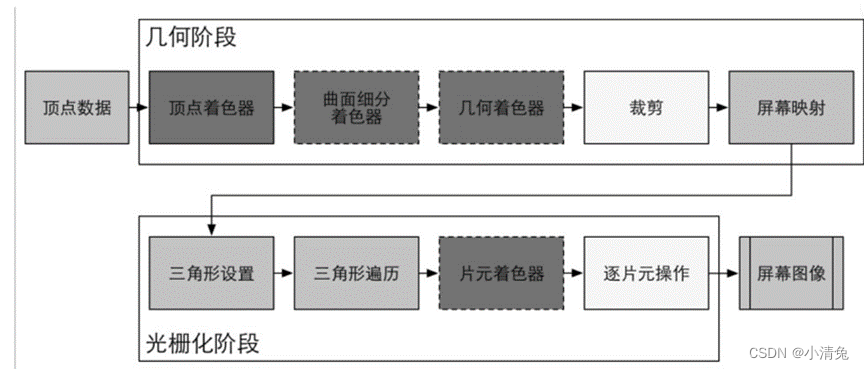As can be seen from the figure, the GPU's rendering pipeline receives vertex data as input. These vertex data are loaded into the video memory by the application stage and then specified by Draw Call. This data is then passed to the vertex shader.
Vertex Shader (Vertex Shader) is fully programmable and is usually used to implement functions such as spatial transformation of vertices and vertex shading. The Tessellation Shader is an optional shader that is used to tessellate primitives. The Geometry Shader is also an optional shader that can be used to perform per-primitive shading operations, or to generate more primitives. The next pipeline stage is clipping. The purpose of this stage is to clip out the vertices that are not within the camera's field of view and to eliminate the patches of certain triangle primitives. This stage is configurable. For example, we can use a custom clipping plane to configure the clipping area, and we can also use instructions to control whether to clip the front or back of the triangle primitive. The last pipeline stage of the geometric concept stage is screen mapping. This stage is not configurable and programmable, and it is responsible for converting the coordinates of each primitive into the screen coordinate system.
As can be seen from the figure, the rendering pipeline of the GPU receives vertex data as input. These vertex data are loaded into the video memory by the application stage, and then specified by Draw Call. This data is then passed to the vertex shader. Vertex Shader (Vertex Shader) is fully programmable, and it is usually used to implement vertex space transformation, vertex coloring and other functions. Tessellation Shader is an optional shader that is used to subdivide primitives. The Geometry Shader is also an optional shader that can be used to perform per-primitive shading operations, or to generate more primitives. The next pipeline stage is clipping. The purpose of this stage is to clip out the vertices that are not within the camera's field of view and to eliminate the patches of certain triangle primitives. This stage is configurable. For example, we can use a custom clipping plane to configure the clipping area, and we can also use instructions to control whether to clip the front or back of the triangle primitive. The last pipeline stage of the geometric concept stage is screen mapping. This stage is non-configurable and non-programmable. It is responsible for converting the coordinates of each primitive into the screen coordinate system.

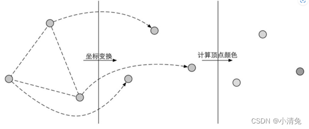
1. The vertex shader (Vertex Shader) is the first stage of the pipeline, and its input comes from the CPU. The processing unit of the vertex shader is a vertex, that is to say, the vertex shader is called once for each vertex input. The vertex shader itself cannot create or destroy any vertices, and it cannot obtain the relationship between vertices. For example, we have no way of knowing whether two vertices belong to the same triangular mesh. But precisely because of this mutual independence, the GPU can use its own characteristics to process each vertex in parallel, which means that the processing speed of this stage will be very fast. The main tasks that the vertex shader needs to complete include: coordinate transformation and per-vertex lighting. Of course, in addition to these two main tasks, the vertex shader can also output data required by subsequent stages. The figure shows the process of coordinate transformation of the vertex position and calculation of the vertex color in the vertex shader.

·Coordinate transformation. As the name suggests, it is to perform some transformation on the coordinates (i.e., position) of the vertices. The vertex shader can change the position of the vertex in this step, which is very useful in vertex animation. For example, we can simulate water, cloth, etc. by changing the position of vertices. But it should be noted that no matter how we change the position of the vertex in the vertex shader, one of the most basic tasks that a vertex shader must complete is to convert the vertex coordinates from model space to homogeneous clipping space. Think about it, will we see code similar to the following in the vertex shader? The

function of the code above is to convert the vertex coordinates into a homogeneous clipping coordinate system, and then usually perform perspective division by the hardware. Finally, the normalized device coordinates (Normalized Device Coordinates, NDC) are obtained. . The figure shows such a conversion process.
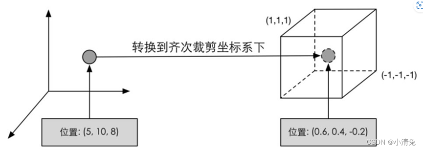It should be noted that the coordinate range given in the figure is NDC used by OpenGL and Unity. Its z component range is between [-1, 1], while in DirectX, the z component range of NDC is [0, 1 ]. Vertex shaders can have different output modes. The most common output path is to rasterize and pass it to the fragment shader for processing.
2. Cropping
Since our scene may be very large, and the camera's field of view may not cover all scene objects, a natural idea is that those objects that are not in the camera's field of view do not need to be processed. Clipping was proposed for this purpose. There are three types of relationship between a primitive and the camera field of view: completely in the field of view, partially in the field of view, and completely outside the field of view. Primitives that are completely in view are passed on to the next pipeline stage, and primitives that are completely out of view are not passed down because they do not need to be rendered. And those primitives that are partly in the field of view need to be processed, which is clipping. For example, if one vertex of a line segment is in view and another vertex is not, the vertex outside the view should be replaced by a new vertex located at the intersection of the line segment and the view boundary. Since we know the vertex position under NDC, that is, the vertex position is within a cube, clipping becomes very simple: only need to clip the primitive into the unit cube. The figure shows such a process.
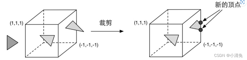Unlike the vertex shader, this step is not programmable, that is, we cannot control the clipping process through programming, but a fixed operation on the hardware, but we can customize a clipping operation for Configure this step.

3. Screen mapping
The coordinates entered in this step are still coordinates in the three-dimensional coordinate system (the range is within the unit cube). The task of screen mapping (ScreenMapping) is to convert the x and y coordinates of each primitive to the screen coordinate system (Screen Coordinates). The screen coordinate system is a two-dimensional coordinate system, which has a lot to do with the resolution we use to display the screen. Suppose, we need to render the scene to a window, the range of the window is from the smallest window coordinates (x1, y1) to the largest window coordinates (x2, y2), where x1< x2 and y1< y2. Since the coordinates we input range from -1 to 1, we can imagine that this process is actually a scaling process, as shown in Figure 2.10. You may ask, what happens to the input z coordinate? Screen mapping does nothing with the input z coordinate. In fact, the screen coordinate system and the z coordinate together form a coordinate system called the window coordinate system (Window Coordinates). These values ​​are passed together to the rasterization stage. The screen coordinates obtained by screen mapping determine which pixel on the screen this vertex corresponds to and how far it is from this pixel.
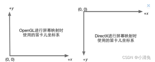
One thing that needs attention is the difference in screen coordinate systems between OpenGL and DirectX. OpenGL regards the lower left corner of the screen as the minimum window coordinate value, while DirectX defines the upper left corner of the screen as the minimum window coordinate value. The figure shows this difference.

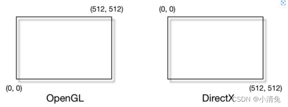
The reason for this difference is that Microsoft's windows all use this coordinate system, because it is consistent with the way we read: left to right, top to bottom, and many image files are also formatted in this way. stored.
Whatever the reason, the difference is made. The message left to us developers is to always be careful about such differences. If you find that the resulting image is inverted, then this is probably the reason.
4. Triangle settings
From this step, it enters the rasterization stage. The information output from the previous stage is the vertex positions in the screen coordinate system and additional information related to them, such as depth value (z coordinate), normal direction, viewing angle direction, etc. The rasterization stage has two most important goals: calculating which pixels each primitive covers, and for those pixels calculating their colors. The first pipeline stage of rasterization is Triangle Setup. This stage computes the information needed to rasterize a triangle mesh. Specifically, the previous stage outputs all the vertices of the triangular mesh, that is, what we get are the two endpoints of each side of the triangular mesh. But if we want to get the pixel coverage of the entire triangular mesh, we must calculate the pixel coordinates on each edge. In order to be able to calculate the coordinate information of the boundary pixels, we need to get the representation of the triangle boundary. Such a process of computing triangular meshes to represent data is called triangle setup. Its output is to prepare for the next stage.

5. Triangle Traversal
The Triangle Traversal stage will check whether each pixel is covered by a triangle mesh. If overwritten, a fragment is generated. The process of finding which pixels are covered by the triangle grid is triangle traversal. This stage is also called Scan Conversion. The triangle traversal stage will determine which pixels are covered by a triangular mesh based on the calculation results of the previous stage, and use the vertex information of the three vertices of the triangular mesh to interpolate the pixels in the entire coverage area. The figure shows the simplified calculation process of the triangle traversal phase.

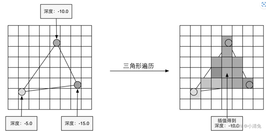
According to the vertex information output by the geometry stage, the pixel position covered by the triangular mesh is finally obtained. The corresponding pixel will generate a fragment, and the state in the fragment is obtained by interpolating the information of the three vertices. The
output of this step is to obtain a fragment sequence. It should be noted that a fragment is not a true pixel, but a collection of states that are used to calculate the final color of each pixel. These states include (but are not limited to) its screen coordinates, depth information, and other vertex information output from the geometry stage, such as normals, texture coordinates, etc.

6. Fragment Shader
Fragment Shader is another very important programmable shader stage. In DirectX, the fragment shader is called a pixel shader (Pixel Shader), but the fragment shader is a more appropriate name, because the fragment at this time is not a real pixel. The previous rasterization stage does not actually affect the color value of each pixel on the screen, but will generate a series of data information to describe how a triangular grid covers each pixel. Each fragment is responsible for storing such a series of data. The stage that really affects the pixels is the next pipeline stage - Per-Fragment Operations. We'll get to that later. The input to the fragment shader is the result of interpolating the vertex information from the previous stage, more specifically, from the data output from the vertex shader. And its output is one or more color values. The figure shows such a process.

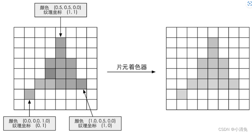Based on the fragment information after interpolation in the previous step, the fragment shader calculates the output color of the fragment.
This stage can complete many important rendering technologies, one of the most important technologies is texture sampling. In order to perform texture sampling in the fragment shader, we usually output the texture coordinates corresponding to each vertex in the vertex shader stage, and then interpolate the texture coordinates corresponding to the three vertices of the triangular mesh through the rasterization stage. The texture coordinates of the fragments it covers can be obtained. While the fragment shader can accomplish many important effects, its limitation is that it can only affect a single fragment. That is, when a fragment shader is executed, it cannot send any of its results directly to its neighbors. The one exception is that the fragment shader has access to derivative information (gradient, or derivative). Interested readers can refer to the extended reading section of this chapter.

7. Fragment-by-fragment operation
Finally, we have reached the last step of the rendering pipeline. Per-Fragment Operations is a term in OpenGL. In DirectX, this stage is called Output-Merger. The word Merger may make it easier for readers to understand the purpose of this step: merging. The names in OpenGL can let readers understand the operation unit of this stage, which is to perform some operations on each fragment. So the question is, what data should be merged? What operations need to be performed?
There are several main tasks in this stage.
(1) Determine the visibility of each fragment. This involves a lot of testing work, such as in-depth testing, template testing, etc. (2) If a fragment passes all the tests, it is necessary to merge or mix the color value of the fragment with the color already stored in the color buffer. It should be noted that the fragment-by-fragment operation stage is highly configurable, that is, we can set the operation details of each step. This will be discussed later. This stage first needs to solve the visibility problem of each fragment. This requires a series of tests. This is like an exam. Only when a fragment passes all the exams can it finally be qualified to negotiate with the GPU. This qualification means that it can be merged with the color buffer. If it doesn't pass one of these tests, then sorry, all the work done to generate this fragment is in vain, because this fragment will be discarded. Poor fragment! The figure shows the operations performed by the simplified fragment-by-fragment operation.

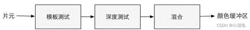
Operations performed in the fragment-by-fragment operation phase. Only after passing all the tests, the newly generated fragments can be mixed with the existing pixel colors in the color buffer, and finally written into the color buffer. The test process is actually a relatively complicated process, and
different The implementation details of graphics interfaces such as OpenGL and DirectX also vary. Here are the implementation processes of the two most basic tests - depth testing and template testing. Understanding these testing procedures will depend on the reader's ability to understand the rendering queue mentioned in the later chapters of this book, especially the problems that arise when dealing with transparency effects. The figure shows a simplified flow chart of depth testing and template testing.

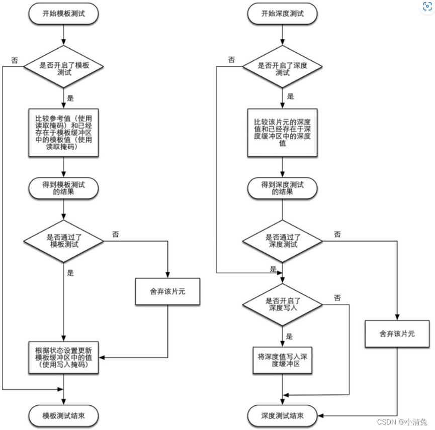
Simplified flow chart of stencil testing and depth testing
Let’s first look at stencil testing (Stencil Test). Related to this is the Stencil Buffer. In fact, the stencil buffer is almost the same thing as the color buffer and depth buffer that we often hear. If the template test is turned on, the GPU will first read (using the read mask) the template value of the fragment position in the template buffer, and then combine this value with the reference value (reference value) read (using the read mask). value), this comparison function can be specified by the developer, for example, discard the fragment when it is less than, or discard the fragment when it is greater than or equal to. If the fragment fails this test, the fragment is discarded. Regardless of whether a fragment passes the stencil test or not, we can modify the stencil buffer according to the stencil test and the following depth test results. This modification operation is also specified by the developer. Developers can set modification operations under different results, for example, the stencil buffer remains unchanged when it fails, and the value of the corresponding position in the stencil buffer is increased by 1 when it passes, etc. Stencil tests are often used to limit the area rendered. In addition, template testing also has some more advanced uses, such as rendering shadows, contour rendering, etc.
If a fragment is lucky enough to pass the template test, then it will go to the next test - the depth test (Depth Test). I believe many readers have heard of this test. This test is also highly configurable. If depth testing is enabled, the GPU will compare the depth value of the fragment with the depth value already in the depth buffer. This comparison function can also be set by the developer, for example, discard the fragment when it is less than, or discard the fragment when it is greater than or equal to. Usually this comparison function is less than or equal to the relationship, that is, if the depth value of this fragment is greater than or equal to the value in the current depth buffer, then it will be discarded. This is because we always want to display only the objects closest to the camera, and those that are obscured by other objects do not need to appear on the screen. If the fragment fails this test, the fragment is discarded. Somewhat different from the stencil test is that if a fragment fails the depth test, it does not have the right to change the value in the depth buffer. And if it passes the test, the developer can also specify whether to use the depth value of this fragment to overwrite the original depth value. This is done by turning on/off depth writing. We will find in later studies that the transparency effect is very closely related to depth testing and depth writing.
Why is merging necessary? We need to know that the rendering process discussed here is drawing one object after another on the screen. The color information of each pixel is stored in a place called the color buffer. Therefore, when we perform this rendering, the color buffer often already has the color result after the last rendering. So, do we use the color obtained from this rendering to completely overwrite the previous result, or do we perform other processing? This is what the merger needs to solve. For opaque objects, developers can turn off the blending operation. In this way, the color value calculated by the fragment shader will directly overwrite the pixel value in the color buffer. But for translucent objects, we need to use blending operations to make the object look transparent. The figure shows a simplified version of the flow chart of the mixing operation.

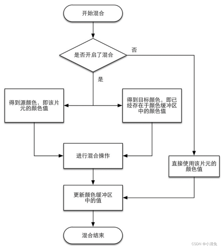
Simplified flowchart of hybrid operation
From the flowchart, we can find that hybrid operation is also highly configurable: developers can choose to turn on/off the hybrid function. If the mixing function is not turned on, the color in the color buffer will be overwritten directly with the color of the fragment, and this is why many beginners find that they cannot get the transparency effect (the mixing function is not turned on). If mixing is turned on, the GPU will take out the source color and target color and mix the two colors. The source color refers to the color value obtained by the fragment shader, while the target color is the color value that already exists in the color buffer. After that, a blending function is used to perform the blending operation. This blending function is usually closely related to the transparent channel, such as addition, subtraction, multiplication, etc. based on the value of the transparent channel. Blending is very similar to the operation of layers in Photoshop: each layer can choose a blending mode, which determines the blending result of this layer and the lower layer, and the picture we see is the mixed picture.
The order of tests given above is not unique, and while it is logical that these tests are run after the fragment shader, for most GPUs they are run as much as possible before the fragment shader is executed these tests. This is understandable. Imagine that when the GPU spends a lot of effort in the fragment shader stage and finally calculates the color of the fragment, it finds that the fragment has not passed these tests at all, that is to say, the fragment is still rejected. If you abandon it, all the calculation costs spent before will be wasted! Figure 2.17 shows such a scenario.

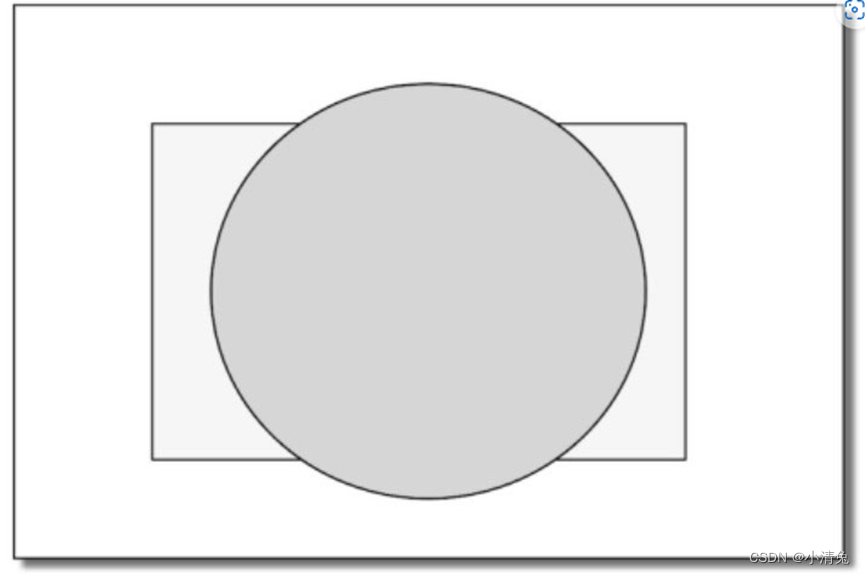
The scene contains two objects: a ball and a cuboid. The drawing sequence is to draw the ball (displayed as a circle on the screen) first, and then draw the cuboid (displayed as a rectangle on the screen). If the depth test is performed after the fragment shader, then when rendering the cuboid, although most of its area is occluded behind the ball, that is, most of the fragments it covers cannot pass the depth test at all, but we still Fragment shaders need to be executed on these fragments, resulting in a huge waste of performance.
As a GPU that wants to fully improve performance, it will want to know which fragments will be discarded as early as possible, so that these fragments do not need to use fragment shaders to calculate their colors. In the rendering pipeline given by Unity, we can also find that the depth test it gives is before the fragment shader. This technology of executing depth testing in advance is often called Early-Z technology. I hope readers will not be confused by this when reading this
. However, if these tests are carried out in advance, the verification results may conflict with some operations in the fragment shader. For example, if we perform a transparency test in the fragment shader, and the fragment fails the transparency test, we will call the API (such as the clip function) in the shader to manually discard it. This results in the GPU being unable to perform various tests in advance. Therefore, modern GPUs will determine whether operations in the fragment shader conflict with look-ahead testing, and if so, disable look-ahead testing. However, this will also cause a performance drop because more fragments need to be processed. This is why transparency testing can cause performance degradation.
After the model elements have gone through the above layers of calculations and tests, they will be displayed on our screen. Our screen displays the color values ​​in the color buffer. However, in order to avoid seeing primitives that are being rasterized, the GPU uses a double buffering strategy. This means that the rendering of the scene happens behind the scenes, in the back buffer. Once the scene has been rendered into the back buffer, the GPU swaps the contents of the back buffer with the front buffer, which is the image previously displayed on the screen. This ensures that the images we see are always continuous.
The summary is as follows:
Although we have talked a lot above, the actual implementation process is far more complicated than what is mentioned above. It should be noted that readers may find that the pipeline names and sequences given here may be different from those seen in some materials. One reason is that the implementation of image programming interfaces (such as OpenGL and DirectX) is not the same. Another reason is that the GPU may have done a lot of optimization at the bottom layer. For example, the depth test mentioned above will be performed before the fragment shader. It seems that Avoid unnecessary calculations. Although the rendering pipeline is relatively complex, Unity, as an excellent platform, encapsulates many functions for us. More often, we only need to set some inputs in a Unity Shader, write vertex shaders and fragment shaders, and set some states to achieve most of the common screen effects. This is the attractive charm of Unity, but the disadvantage is that the encapsulation will lead to a decrease in the degree of freedom of programming, making many beginners lose their way, unable to grasp the principles behind it, and often unable to find the cause of the error when there is a problem , this is a common encounter when learning Unity Shader. The rendering pipeline is closely related to almost all chapters of this book. If readers still cannot fully understand the rendering pipeline at this time, they can continue to learn. However, if readers find that some settings or codes cannot be understood during the learning process, they can continue to refer to the content of this chapter and I believe they will have a deeper understanding.

Unity’s basic lighting

The emissive part is represented by cmissive.
This section describes how much radiation a surface itself emits in a given direction. It should be noted that if global illumination technology is not used, these self-illuminating surfaces will not actually illuminate the surrounding objects, but they will just look brighter themselves.
Light can also be emitted directly from the light source into the camera without being reflected by any object. The standard lighting model uses self-illumination to calculate this contribution. Its calculation is also very simple, that is, the self-illuminating color of the material is directly used: cemissive=memissive Usually in real-time rendering, the self-illuminating surface often does not illuminate the surrounding surface, that is to say, the object does not used as a light source.

·The specular part is represented by cspecular. This section describes how much radiation will be scattered by the surface in the direction of perfect specular reflection when light hits a model surface from a light source.

The specular reflection here is an empirical model, that is, it does not exactly correspond to the specular phenomenon in the real world. It can be used to calculate the rays that are reflected along the direction of full specular reflection, which can make objects look shiny, such as metal materials.
Calculating specular reflection requires knowing a lot of information, such as surface normal, viewing angle direction, light source direction, reflection direction, etc. Using the

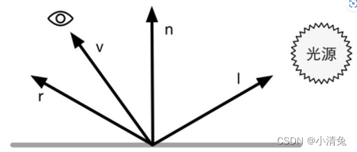
Phong model to calculate specular reflection,
among these four vectors, we actually only need to know 3 of them. The fourth vector, the reflection direction, can be calculated from other information.
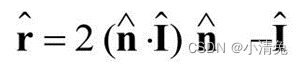In this way, we can use the Phong model to calculate the specular reflection part:

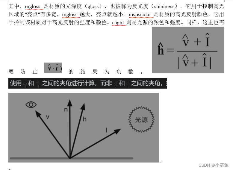
The formula of the Blinn model is as follows:
In hardware implementation, if the camera and light source are far enough from the model , the Blinn model will be faster than the Phong model, because at this time it can be considered that both [illustration] and [illustration] are constant values, so [illustration] will be a constant. However, when [illustration] or [illustration] is not constant, the Phong model may be faster instead. It should be noted that both lighting models are empirical models, that is, we should not consider the Blinn model to be an approximation of the "correct" Phong model. In fact, in some cases, the Blinn model fits the experimental results better.

·Diffuse part is represented by cdiffuse. This section describes how much radiation the surface scatters in each direction when light hits it from a light source.

Diffuse lighting is used to model radiance that is randomly scattered in all directions by the surface of an object. In diffuse reflection, the position of the viewing angle is unimportant because the reflection is completely random, so the distribution can be considered to be the same in any reflection direction. However, the angle of the incoming light is important. Diffuse lighting complies with Lambert's law: the intensity of reflected light is proportional to the cosine of the angle between the surface normal and the direction of the light source. Therefore, the diffuse part is calculated as follows:
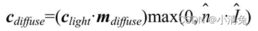
is the surface normal
which is the unit vector pointing towards the light source, mdiffuse is the diffuse color of the material and clight is the light color. It should be noted that we need to prevent the result of the point multiplication of the normal and the direction of the light source from being negative. To do this, we use the function that takes the maximum value to intercept it to 0. This can prevent the object from being illuminated by the light source from behind. .

·The ambient light (ambient) part is represented by cambient. It is used to describe all other indirect lighting.
Although the standard lighting model focuses on describing direct lighting, in the real world, objects can also be illuminated by indirect light. Indirect illumination means that light usually reflects between multiple objects and finally enters the camera. That is, before the light enters the camera, it has been reflected by more than one object. For example, if you place a light gray sofa on the red carpet, there will also be red at the bottom of the sofa. These reds are part of the light reflected by the red carpet and then bounced to the sofa. In the standard lighting model, we use something called ambient light to approximate indirect lighting. The calculation of ambient light is very simple, it is usually a global variable, that is, all objects in the scene use this ambient light. The part of calculating ambient light: ambient=gambient
pixel-by-pixel or vertex-by-vertex
We have given the mathematical formulas used by the basic lighting model, so where do we calculate these lighting models? Generally speaking, we have two options: calculate in the fragment shader, also known as per-pixel lighting (per-pixel lighting); calculate in the vertex shader, also known as per-vertex lighting (per-vertex lighting). lighting). In pixel-by-pixel lighting, we will get its normal based on each pixel (it can be obtained by interpolating the vertex normal, or it can be obtained by sampling from the normal texture), and then calculate the lighting model . This technique of interpolating vertex normals between patches is called Phong shading, also known as Phong interpolation or normal interpolation shading techniques. This is different from the Phong lighting model we talked about earlier.
The opposite is per-vertex lighting, also known as Gouraud shading. In per-vertex lighting, we calculate lighting on each vertex, then perform linear interpolation within the rendering primitive, and finally output it as a pixel color. Since the number of vertices is often much smaller than the number of pixels, the calculation amount of per-vertex lighting is often smaller than that of per-pixel lighting. However, since per-vertex lighting relies on linear interpolation to obtain pixel lighting, problems will arise when there are non-linear calculations in the lighting model (such as when calculating specular reflection). We will see this situation in later chapters. Moreover, since per-vertex lighting interpolates the vertex color within the rendering primitive, this will cause the color inside the rendering primitive to always be darker than the highest color value at the vertex, which will produce obvious angular phenomena in some cases. .
Summary:
Although the standard lighting model is only an empirical model, that is to say, it does not fully conform to the lighting phenomena in the real world. However, due to its ease of use, calculation speed and better results, it is still widely used. And because of its widespread use, this standard lighting model has many different names. For example, some sources call it the Phong lighting model because Bui Tuong Phong first proposed the basic idea of ​​using the sum of diffuse reflection and specular reflection to model reflected lighting, and also proposed an empirical method for calculating specular reflection. method (the Lambert model for calculating diffuse illumination had already been proposed at that time). Then, because Blinn's method simplifies calculations and is faster in some cases, we call this model the Blinn-Phong lighting model. But this model has many limitations. First of all, there are many important physical phenomena that cannot be represented by the Blinn-Phong model, such as Fresnel reflection. Secondly, the Blinn-Phong model is isotropic, which means that when we rotate the surface with a fixed viewing angle and light source direction, the reflection will not change in any way. But some surfaces have anisotropic reflective properties, such as brushed metal, hair, etc.

Diffuse and specular lighting models

Basic textures (leaflet, bump, gradient, mask)

Transparency effect (transparency test, transparency mixing, translucency, double-sided transparent and non-transparent stickers)

Unity's standard shader

Advanced textures (cube textures, render textures, degree textures, (texture animation, vertex animation), screen post-processing (screen brightness saturation contrast, edge detection, Gaussian blur, Bloom effect, motion blur))

Depth and normal textures (get depth and normal textures, motion blur 2, edge detection 2, global fog effect)

Non-photorealistic rendering (cartoons, sketches)

Use noise (ablation, water wave, global fog effect 2)

Note:
Check the code part by yourself.
Link: https://pan.baidu.com/s/1YEWZHW-21nKPBIIX2q8-1w?pwd=g7nd
Extraction code: g7nd

Basic math for Unity shaders

1. Cartesian coordinate system

We use mathematics mostly to calculate variables such as position, distance, and angle. Most of these calculations are performed in the Cartesian coordinate system.

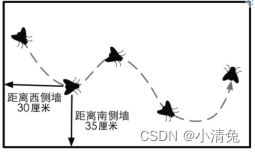
The Carr coordinate system originated from Descartes' observation of the trajectory of a fly on the ceiling. Descartes discovered that the distance of a fly from different walls can be used to describe its current position.

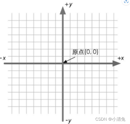
Two-dimensional Cartesian coordinate system
A two-dimensional Cartesian coordinate system contains two parts of information:
·A special position, That is, the origin, which is the center of the entire coordinate system.
Two mutually perpendicular vectors passing through the origin, namely the x-axis and the y-axis. These axes are also called the basis vectors of the coordinate system

2. Point and vector

A point is a position in n-dimensional space (two-dimensional and three-dimensional spaces are mainly used in games). It has no concepts such as size and width. In the Cartesian coordinate system, we can use 2 or 3 real numbers to represent the coordinates of a point. For example, P=(Px, Py) represents a point in two-dimensional space, and P=(Px, Py, Pz) represents a three-dimensional point. point in space.
The definition of vector (also known as vector) is a bit more complicated. To mathematicians, a vector is just a sequence of numbers. You may want to ask, isn't the expression of point also a string of numbers? Yes, but the purpose of vectors is to distinguish them from scalars. Generally speaking, a vector refers to a directed line segment in n-dimensional space that contains magnitude and direction. The velocity we usually talk about is a typical vector. For example, the speed of this car is 80km/h south (south indicates the direction of the vector, and 80km/h indicates the module of the vector). A scalar quantity has only a modulus but no direction. The distance often mentioned in life is a kind of scalar quantity. For example, my home is only 200m away from the school (200m is a scalar quantity).
Specifically.
·The module of a vector refers to the length of this vector. The length of a vector can be any nonnegative number.
·The direction of a vector describes where the vector points in space. Vectors are represented similarly to points. We can use v=(x, y) to represent a two-dimensional vector, v=(x, y, z) to represent a three-dimensional vector, and v=(x, y, z, w) to represent a four-dimensional vector. To facilitate explanation, we use different writing and printing styles for different types of variables.
·For scalars, we use lowercase letters to represent them, such as a, b, x, y, z, θ, α, etc.
·For vectors, we use lowercase bold letters to represent them, such as a, b, u, v, etc.
·For matrices to be learned later, we use uppercase bold letters to represent them, such as A, B, S, M, R, etc.

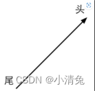
A vector is usually represented by an arrow. We sometimes talk about the head and tail of a vector. The head of a vector refers to the endpoint of its arrow, while the tail refers to the other endpoint.
From the definition of a vector, it only has two attributes: module and direction, and no position information. This sounds difficult to understand, but in fact we always deal with such vectors in life. For example, when we talk about the speed of an object, we may say "the thief is running south at a speed of 100km/h" (catch him quickly!), here "going south at a speed of 100km/h" It can be represented by a vector. Typically, a vector is used to represent a displacement relative to a point, that is, it is a relative quantity. As long as the magnitude and direction of the vector remain the same, it is the same vector no matter where it is placed.
The difference between a point and a vector
: A point is a position in space that has no size, while a vector is a quantity that has a modulus and direction but no position. From here, points and vectors have different meanings. However, the representation is very similar.
Vector and scalar multiplication/division

A vector can also be divided by a non-zero scalar. This is equivalent to multiplying by the reciprocal of this scalar:

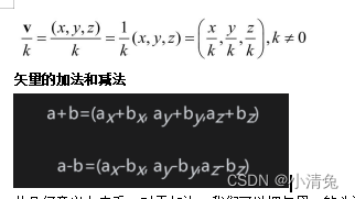
From a geometric point of view, for addition, we can connect the head of vector a to the tail of vector b, and then draw a vector from the tail of a to the head of b to get the vector after adding a and b. In other words, if we perform a position offset a from a starting point, and then perform a position offset b, it is equivalent to a position offset of a+b. This is called the triangle rule for vector addition. Vector subtraction is similar to

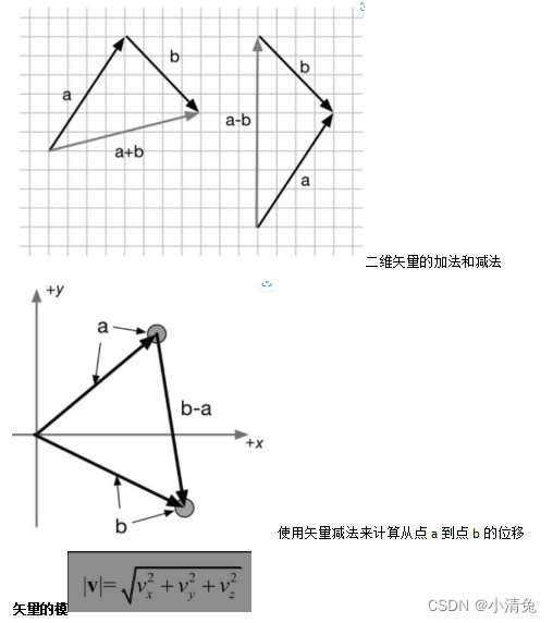
Unit vector
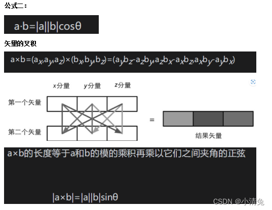
Dot product of vectors

Dot product has some very important properties. In the calculation of Shader, we will often use these properties to help calculate.
Property 1: Dot product can be combined with scalar multiplication. The "combination" above means that one of the operands of the dot product can be the result of another operation, namely the multiplication of a vector and a scalar. The formula is as follows: (ka)·b= a·(kb)=k(a·b) In other words, the result of scaling one of the vectors in the dot product is equivalent to scaling the final dot product result.
Property 2: Dot product can be combined with vector addition and subtraction, similar to Property 1. "Combined" here means that the operands of the dot product can be the result of vector addition or subtraction. Expressed as a formula: a·(b+ c)= a·b+ a·c
Property 3: The result of the dot product of a vector and itself is the square of the module of the vector. This can be easily verified from the formula: v ·v=vxvx+vyvy+vzvz=|v|2
This means that we can directly use the dot product to find the module of the vector without using the module calculation formula. Of course, we need to perform the square root operation on the dot product result to get the real module. But in many cases, we just want to compare the lengths of two vectors, so we can directly use the result of the dot product. After all, the square root operation requires a certain amount of performance. Now it's time to look at another representation of dot product. This method is based on the perspective of trigonometric algebra. This representation method is more geometric because it can clearly emphasize the angle between two vectors.

3. Matrix

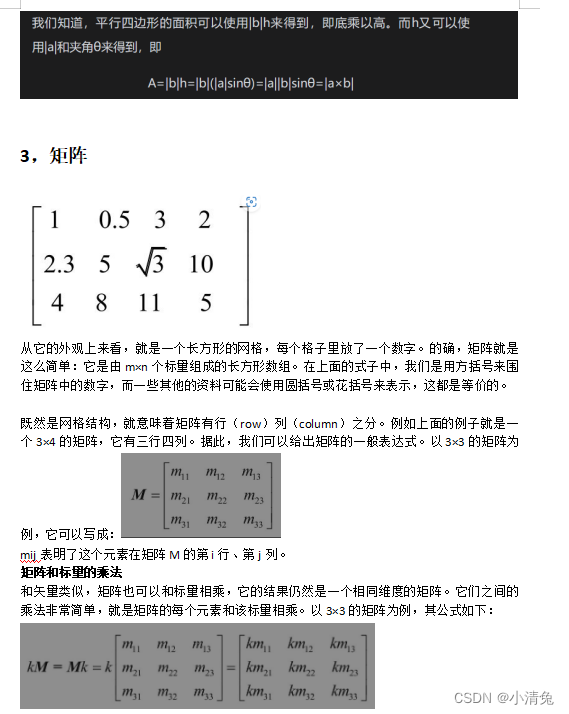
Matrix and matrix multiplication
What if the rows and columns of the two matrices do not meet the above regulations? So I'm sorry, these two matrices cannot be multiplied because the multiplication between them is not defined (of course, readers can define a new multiplication by themselves, but it is not certain whether mathematicians will buy it. ). So why are there the above regulations? We will understand it naturally when we understand the operation process of matrix multiplication. We first give a mathematical expression that seems very complicated and difficult to understand (readers will find that it is not that difficult to understand when the intuitive expression is given): Let there be an r×n matrix A and an n×c matrix B. , multiplying them will result in an r×c matrix C=AB. Then, each element cij in C is equal to the vector corresponding to the i-th row of A

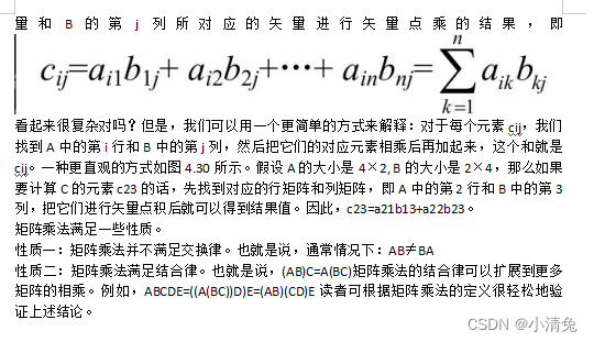
4. Geometric meaning of matrix, (transformation)

What is transformation
Transformation refers to the process in which we convert some data, such as points, direction vectors, and even colors, in some way. In the field of computer graphics, transformations are very important. Although the operations we can perform through transformation are limited, these operations are enough to establish transformation's pivotal position in the field of graphics.
Let’s first look at a very common type of transformation—linear transform. Linear transformations are those that preserve vector additions and scalar multiplications. Using mathematical formulas to express these two conditions is:

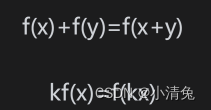
It can be seen that the results obtained by the two operations are different. Therefore, we cannot use a 3×3 matrix to represent a translation transformation. This is something we don't want to see. After all, translation transformation is a very common transformation. In this way, there is an affine transform. Affine transformation is a type of transformation that combines linear transformation and translation transformation. Affine transformation can be represented by a 4×4 matrix. To do this, we need to extend the vector into a four-dimensional space, which is a homogeneous space.
Homogeneous coordinates
A homogeneous coordinate is a four-dimensional vector. So, how do we convert three-dimensional vectors into homogeneous coordinates? For a point, converting from three-dimensional coordinates to homogeneous coordinates is to set its w component to 1, and for a direction vector, its w component needs to be set to 0. Such a setting will cause that when a point is transformed using a 4×4 matrix, translation, rotation, and scaling will be applied to the point. But if it is used to transform a direction vector, the translation effect will be ignored. We can understand the reasons for these differences from the following content:
Decomposing the basic transformation matrix
We already know that a 4×4 matrix can be used to represent translation, rotation and scaling. We call the transformation matrix representing pure translation, pure rotation and pure scaling the basic transformation matrix. These matrices have something in common,

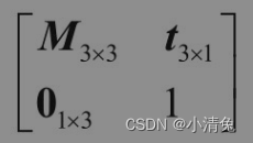
Among them, the matrix M3×3 in the upper left corner is used to represent rotation and scaling, t3×1 is used to represent translation, 01×3 is a zero matrix, that is, 01×3=[0 0 0], and the element in the lower right corner is the scalar 1.
Translation matrix
The translation transformation has no effect on the direction vector. This is easy to understand. As we said when we were learning vectors, a vector has no position attribute, which means it can be located at any point in space, so changes in position (i.e. translation) should not have an impact on the four-dimensional vector. .
Scaling matrix
If the scaling coefficient kx=ky=kz, we call such scaling a uniform scale, otherwise it is called a nonuniform scale. Visually, uniform scaling expands the entire model, while non-uniform scaling stretches or squeezes the model. More importantly, uniform scaling does not change the angle and scale information, while non-uniform scaling changes the angle and scale associated with the model. For example, when transforming normals, if there is non-uniform scaling, if you directly use the transformation matrix used to transform vertices, you will get wrong results.
If we want to scale in any direction, we need to use a compound transformation. The main idea of ​​one of the methods is to first transform the scaling axis into a standard coordinate axis, then perform scaling along the coordinate axis, and then use the inverse transformation to obtain the original scaling axis orientation.
Rotation Matrix
The inverse of a rotation matrix is ​​the transformation matrix obtained by rotating the opposite angle. The rotation matrix is ​​an orthogonal matrix, and the concatenation of multiple rotation matrices is also orthogonal.
Compound transformation
We can combine translation, rotation and scaling to form a complex transformation process. For example, you can first scale a model to a size of (2, 2, 2), then rotate it 30° around the y-axis, and finally translate it 4 units toward the z-axis. Composite transformations can be achieved through the concatenation of matrices. The above transformation process can be calculated using the following formula:
pnew=MtranslationMrotationMscalθ oldp
Since we are using a column matrix above, the reading order is from right to left, that is, scaling transformation is performed first, then rotation transformation is performed, and finally translation transformation is performed. It should be noted that the result of the transformation depends on the order of transformation. Since matrix multiplication does not satisfy the commutative law, the order of matrix multiplication is important. That is to say, the results obtained by different transformation orders may be the same. Imagine asking a reader to take a step forward and then turn left, remembering where they are. Then return to the original position, this time turn left and then take a step forward, the position obtained is different from the last time. The essence is that the multiplication of matrices does not satisfy the commutative law, so the results obtained by different multiplication sequences are different.
In most cases, we agree that the order of transformation is to scale first, then rotate, and finally translate'
'

5. Coordinate space

Transformation of coordinate space
We first need to do some mathematical preparation for the following content. In the rendering pipeline, we often need to convert a point or direction vector from one coordinate space to another coordinate space. How is this process achieved? Let us generalize the problem. We know that in order to define a coordinate space, we must specify the location of its origin and the directions of the three coordinate axes. And these values ​​are actually relative to another coordinate space (readers need to remember that everything is relative). In other words, coordinate spaces will form a hierarchical structure - each coordinate space is a subspace of another coordinate space, and conversely, each space has a parent coordinate space. Transforming coordinate space is actually transforming points and vectors between parent space and subspace. Assume that there is a parent coordinate space P and a child coordinate space C. We know the origin position of the child coordinate space in the parent coordinate space and the 3 unit coordinate axes. We generally have two requirements: one requirement is to convert the point or vector Ac represented in the child coordinate space to the representation Ap in the parent coordinate space, and the other requirement is the other way around, that is, to convert the point or vector Ac represented in the parent coordinate space The vector Bp is converted to the representation Bc in the sub-coordinate space. We can use the following formula to express these two requirements:

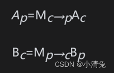
Among them, Mc→p represents the transformation matrix from the child coordinate space to the parent coordinate space, and Mp→c is its inverse matrix (ie, reverse transformation). So, the question now is, how to solve these transformation matrices? In fact, we only need to solve for one of the two, and the other matrix can be obtained by inverting the matrix. Next, we will explain how to find the transformation matrix Mc→p from the child coordinate space to the parent coordinate space. First, let's review a seemingly simple question: when given a coordinate space and a point (a, b, c), how do we know the position of the point?
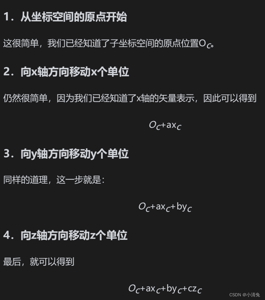
We can determine its position through 4 steps:
(1) Start from the origin of the coordinate space;
(2) Move a unit in the x-axis direction.
(3) Move b units in the y-axis direction
(4) Move c units in the z-axis direction.
It should be noted that the above steps are just our imagination, and this point has not actually moved. The above steps seem to be simple, and the transformation of the coordinate space is contained in the above four steps. Now, we know the representations xc, yc, zc of the three coordinate axes of the sub-coordinate space C in the parent coordinate space P, as well as the position of its origin Oc. When a point Ac=(a, b, c) in the sub-coordinate space is given, we can also follow the above four steps to determine its position Ap in the parent coordinate space: model space (model space),
such
as As its name suggests, it is related to a model or object. Sometimes model space is also called object space or local space. Each model has its own independent coordinate space. When it moves or rotates, the model space will also move and rotate with it. If we think of ourselves as models in the game, when we move in the office, our model space also moves with it. When we turn around, our own front, rear, left, and right directions are also changing.
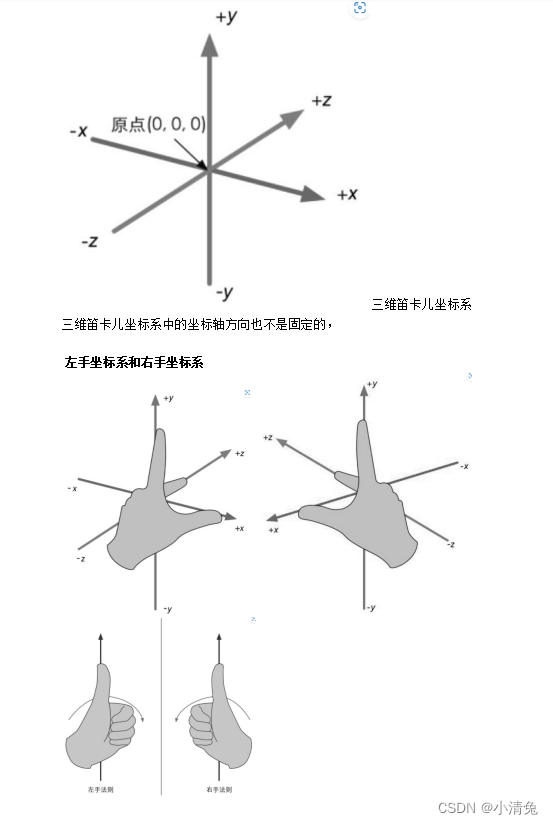
In the model space, we often use some directional concepts, such as "forward", "back", "left", "right", "up" and "down". In this book, we refer to these directions as natural directions. Coordinate axes in model space typically use these natural directions. As we mentioned in Section 4.2.4, Unity uses a left-handed coordinate system in the model space. Therefore, in the model space, the +x axis, +y axis, and +z axis correspond to the right, upper, and front sides of the model respectively. Towards. It should be noted that the correspondence between the x-axis, y-axis, z-axis and the natural direction in the model coordinate space is not necessarily the above-mentioned relationship, but since Unity uses such a convention, this book will use this method. We can click on any object in the Hierarchy view to see the three coordinate axes of their corresponding model space.
The origin and coordinate axes of the model space are usually determined by the artist in the modeling software. When imported into Unity, we can access the model's vertex information in the vertex shader, which contains the coordinates of each vertex. These coordinates are defined relative to the origin in model space (usually located at the center of gravity of the model).
World Space World
space is a special coordinate system because it establishes the largest space we care about. Some readers may point out that space can be infinite, so how can there be such a thing as "maximum"? The maximum mentioned here refers to a macro concept, that is to say, it is the outermost coordinate space that we are concerned about. Take our farm game as an example. In this game, the world space refers to the farm. We don’t care where the farm is. In this virtual game world, the farm is the largest space concept. World space can be used to describe absolute positions (more serious readers may remind me again that there are no absolute positions. Yes, but I believe readers can understand what absolute means here). In this book, absolute position refers to the position in the world coordinate system. Typically, we place the origin of world space at the center of game space.
View space
View space is also called camera space. Observation space can be considered a special case of model space - among all models there is a very special model, that is, the camera (although the camera itself is usually invisible), and its model space deserves our separate discussion. That is the observation space.

The camera determines the perspective from which we render the game. In the observation space, the camera is located at the origin. Similarly, the choice of its coordinate axis can be arbitrary, but since this book mainly discusses Unity, the coordinate axis selection of the observation space in Unity is: +x axis points to the right. , the +y axis points up and the +z axis points behind the camera. Readers may find it strange here. The +z axis in the model space and world space we discussed before refers to the front of the object. Why is it different here? This is because Unity uses a left-handed coordinate system in both model space and world space, while a right-handed coordinate system is used in observation space. This is in line with the OpenGL tradition. In such an observation space, the front of the camera points in the -z direction. This change between the left and right hand coordinate systems rarely affects our programming in Unity, because Unity does a lot of the underlying work of rendering for us, including many coordinate space conversions. However, if readers need to call interfaces such as Camera.camera ToWorldMatrix and Camera.worldToCameraMatrix to calculate the position of a model in the observation space by themselves, they should be careful about this difference.
One last thing to remind readers is that observation space and screen space (see Section 4.6.8 for details) are different. Observation space is a three-dimensional space, while screen space is a two-dimensional space. The conversion from observation space to screen space requires an operation, which is the second step of projection vertex
transformation, which is to transform the vertex coordinates from world space to observation space. This transformation is often called the view transform.
In order to get the position of the vertex in the observation space, we can have two methods. One method is to calculate the representation of the three coordinate axes of the observation space in world space.
Here we use the second method. From the Transform component, we can know that the camera's transformation in world space is first rotated by (30, 0, 0), and then translated by (0, 10, -10). Clipping
space
The vertices are then converted from the observation space to the clip space (clip space, also known as the homogeneous clip space). The matrix used for transformation is called the clip matrix, also known as the projection matrix. . The goal of clipping space is to easily crop rendering primitives: primitives that are completely inside this space will be retained, and primitives that are completely outside this space will be eliminated, and those that intersect with the boundaries of this space will be eliminated. The primitives will be cropped. So, how is this space determined? The answer is determined by the view frustum.

The projection matrix serves two purposes.
· The first is to prepare for the projection. This is a confusing point. Although the name of the projection matrix contains the word projection, it does not perform real projection work, but prepares for projection. The real projection occurs later in the homogeneous division process. After the transformation of the projection matrix, the w component of the vertex will have a special meaning.
The second is to scale the x, y, z components. We mentioned above that it would be troublesome to directly use the six clipping planes of the viewing frustum to perform clipping. After scaling the projection matrix, we can directly use the w component as a range value. If the x, y, and z components are all within this range, it means that the vertex is within the clipping space.

6. Normal transformation

Normal (normal), also known as normal vector (normal vector). Above we've seen how to use a transformation matrix to transform a vertex or a direction vector, but normals are a kind of direction vector that we need special treatment for. In games, a vertex of a model often carries additional information, and the vertex normal is one of the pieces of information. When we transform a model, not only its vertices need to be transformed, but also the vertex normals need to be transformed in order to calculate lighting, etc. in subsequent processing (such as fragment shaders).
In general, points and most direction vectors can be transformed from coordinate space A to coordinate space B using the same 4×4 or 3×3 transformation matrix MA→B. But when transforming the normal, if you use the same transformation matrix, you may not be able to ensure that the verticality of the normal is maintained. Let’s take a look at why this problem occurs.
Let’s first take a look at another type of direction vector—tangent, also known as tangent vector. Similar to normals, tangents are often also a type of information carried by model vertices. It is usually aligned with texture space and is perpendicular to the normal direction,
the tangent and normal to the vertex. The tangent and the normal are perpendicular to each other
. Since the tangent is calculated from the difference between two vertices, we can directly transform the tangent using the transformation matrix used to transform the vertices. Assume that we use a 3×3 transformation matrix MA→B to transform the vertices (note that the transformation matrices involved here are all 3×3 matrices, and translation transformations are not considered. This is because tangents and normals are both direction vectors, not will be affected by translation), the transformed tangent can be obtained directly from the following formula: TB=MA→BTA
where TA and TB represent the tangent directions under coordinate space A and coordinate space B respectively. But if you directly use MA→B to transform the normal, the new normal direction may not be perpendicular to the surface.

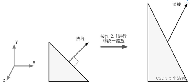
When performing non-uniform scaling, if you use the same transformation matrix to transform the vertex to transform the normal, it will Getting wrong results, i.e. the transformed normal direction is no longer perpendicular to the plane
So, which matrix should be used to transform the normals? We can derive this matrix from the mathematical constraints. We know that the tangent TA and normal NA of the same vertex must satisfy the vertical condition, that is, TA·NA=0. Given the transformation matrix MA→B, we already know that TB=MA→BTA. We now want to find a matrix G to transform the normal NA so that the transformed normal is still perpendicular to the tangent. That is, TB·NB=(MA→BTA)·(GNA)=0. After some derivation of the above formula, we can get

Since TA·NA=0, if, then the above formula can be established. In other words, if you use the inverse transpose matrix of the original transformation matrix to transform the normal, you can get the correct result.
It is worth noting that if the transformation matrix MA → B is an orthogonal matrix, then [ , that is, we can directly transform the normal using the transformation matrix used to transform the vertices. If the transformation consists only of rotation transformations, then this transformation matrix is ​​an orthogonal matrix. And if the transformation only includes rotation and uniform scaling, but not non-uniform scaling, we use the uniform scaling coefficient k to obtain the inverse transpose matrix of the transformation matrix MA→B. This avoids the process of computing the inverse matrix. If the transformation includes a non-uniform transformation, then we have to solve the inverse matrix to get the matrix of transformed normals.

7. Built-in variables of Unityshadwer

1. Transformation matrix

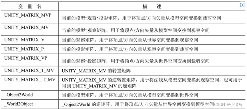
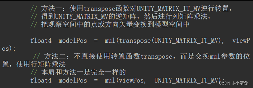
One of the matrices is quite special, namely the UNITY_MATRIX_T_MV matrix. Many readers who are not familiar with mathematics do not understand what this matrix is ​​used for. If readers have carefully read the matrix section, they should also remember a very attractive matrix type-orthogonal matrix. For an orthogonal matrix, its inverse matrix is ​​the transposed matrix. Therefore, if UNITY_MATRIX_MV is an orthogonal matrix, then UNITY_MATRIX_T_MV is its inverse matrix, that is, we can use UNITY_MATRIX_T_MV to transform the vertices and direction vectors from observation space to model space. So the question is, when is UNITY_MATRIX_MV an orthogonal matrix? Readers can find the answer from Section 4.5. To sum up, if we only consider the three transformations of rotation, translation and scaling, if the transformation of a model only includes rotation, then UNITY_MATRIX_MV is an orthogonal matrix. This condition seems a bit harsh. We can relax the condition a little more. If it only includes rotation and uniform scaling (assuming the scaling coefficient is k), then UNITY_MATRIX_MV is almost an orthogonal matrix. Why almost? Because uniform scaling may cause the vector length of each row (or column) to be not 1, but k, which does not comply with the characteristics of an orthogonal matrix, but we can turn it into a positive value by dividing by this uniform scaling coefficient. intersection matrix. In this case, the inverse matrix of UNITY_MATRIX_MV is And, if we only transform the direction vector, the conditions can be broadened, that is, we do not need to consider whether there is a translation transformation, because the translation has no effect on the direction vector. Therefore, we can intercept the first three rows and first three columns of UNITY_MATRIX_T_MV to transform the direction vector from observation space to model space (provided that only rotation transformation and unified scaling exist). For direction vectors, we can normalize them before use to eliminate the effect of uniform scaling.
There is another matrix that needs to be explained, that is the UNITY_MATRIX_IT_MV matrix. We already know in Section 4.7 that the transformation of the normal requires the use of the inverse transpose matrix of the original transformation matrix. Therefore UNITY_MATRIX_IT_MV can transform the normal from model space to observation space. But as long as we do a little trick, it can also be used to directly obtain the inverse matrix of UNITY_MATRIX_MV - we just need to transpose it. Therefore, in order to transform the vertices or direction vectors from observation space to model space, we can use code similar to the following:

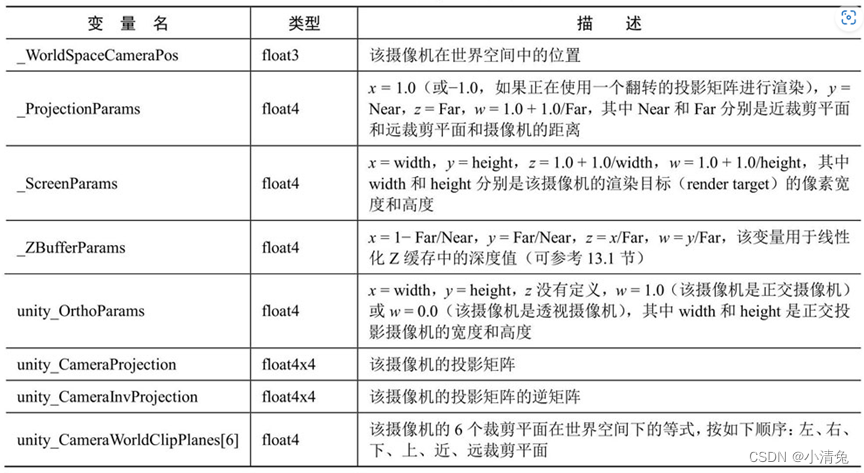
2. Camera and screen parameters

Rendering optimization in unity

1. Characteristics of mobile platforms
Compared with PC platforms, the GPU architecture on mobile platforms is very different. Due to the limitations of processing resources and other conditions, the GPU architecture on mobile devices focuses on using as small a bandwidth and functions as possible, which also brings about many phenomena that are completely different from those on the PC platform. For example, in order to remove those hidden surfaces as much as possible and reduce overdraw (that is, a pixel is drawn multiple times), PowerVR chips (commonly used in iOS devices and some Android devices) use tile-based deferred rendering (Tiled-based Deferred Rendering (TBDR) architecture, all rendered images are loaded into tiles, and then the hardware finds the visible fragments, and only these visible fragments will execute the fragment shader. Other tile-based GPU architectures, such as Adreno (Qualcomm chips) and Mali (ARM chips), will use Early-Z or similar technology to perform a low-precision depth detection to eliminate those tiles that do not need to be rendered. Yuan. There are also some GPUs, such as Tegra (Nvidia's chip), which use traditional architecture designs, so on these devices, overdraw is more likely to cause a performance bottleneck.
2. Factors affecting rendering
First of all, before learning how to optimize, we must understand the factors that affect game performance so that we can prescribe the right medicine. For a game, it mainly requires the use of two computing resources: CPU and GPU. They work together to make our game work at the expected frame rate and resolution. Among them, the CPU is mainly responsible for ensuring the frame rate, and the GPU is mainly responsible for some resolution-related processing. Based on this, we can divide the main causes of game performance bottlenecks into the following aspects.
(1) CPU. ·
Excessive draw calls.
Complex scripts or physics simulations.
(2) (2) GPU. ·Vertex processing.
➢ Too many vertices.
➢ Excessive vertex-by-vertex calculations.
·Fragment processing.
➢ Too many fragments (may be caused by resolution or overdraw).
➢ Excessive piece-by-piece calculations.
(3) Bandwidth.
Large, uncompressed textures are used.
· Framebuffer with too high resolution.

(1) CPU optimization.
· Use batch processing technology to reduce the number of draw calls.
(2) GPU optimization.
• Reduce the number of vertices that need to be processed.
➢ Optimize geometry.
➢ Use the LOD (Level of Detail) technology of the model.
➢ Use Occlusion Culling technology.
·Reduce the number of fragments that need to be processed
➢ Control the drawing order.
➢ Be wary of transparent objects.
➢ Reduce realtime lighting.
• Reduced computational complexity.
➢ Use Shader’s LOD (Level of Detail) technology.
➢ Code optimization.
(3) Save memory bandwidth. ·
Reduce texture size.
· Take advantage of resolution scaling

3. Unity performance optimization analysis tool


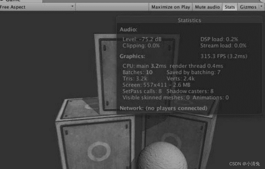
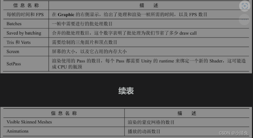
One of the most obvious differences is that the display of the number of draw calls has been removed and the display of the number of batch processing has been added. Batches and Saved by batching make it easier for developers to understand the optimization results of batch processing. Of course, if we want to view the number of draw calls and other more detailed data, we can view it through the performance analyzer of the Unity editor.

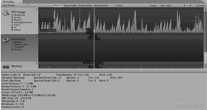
The performance analyzer displays most of the information provided in the rendering statistics window, for example, the green line shows the number of batches, the blue line shows the number of Passes, etc., and also gives a lot of other very useful information, such as draw The number of calls, the number of dynamic batches/static batches, the number of rendering textures and memory usage, etc.
talk about the frame debugger

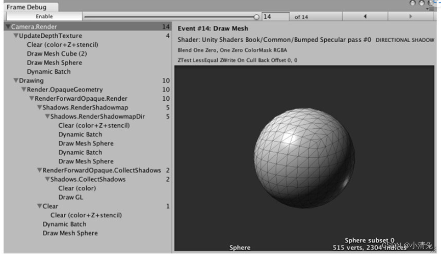
. With the help of Unity's three powerful tools: rendering statistics window, analyzer and frame debugger, we can get a lot Useful optimization information. However, many data such as rendering time are based on the current development platform, rather than the results on the real machine. In fact, Unity is working with hardware manufacturers to first make Tegra-powered devices appear in Unity's performance profiler. We have reason to believe that in subsequent Unity versions, performance analysis of mobile devices directly in Unity will no longer be a dream. However, before this dream can be realized, we still need the help of some external performance analysis tools

4. Reduce drawcalls

最常看到的优化技术大概就是批处理（batching）了。批处理的实现原理就是为了减少每一帧需要的draw call数目。为了把一个对象渲染到屏幕上，CPU需要检查哪些光源影响了该物体，绑定shader并设置它的参数，再把渲染命令发送给GPU。当场景中包含了大量对象时，这些操作就会非常耗时。一个极端的例子是，如果我们需要渲染一千个三角形，把它们按一千个单独的网格进行渲染所花费的时间要远远大于渲染一个包含了一千个三角形的网格。在这两种情况下，GPU的性能消耗其实并没有多大的区别，但CPU的draw call数目就会成为性能瓶颈。因此，批处理的思想很简单，就是在每次面对draw call时尽可能多地处理多个物体

Unity supports two batch processing methods: one is dynamic batch processing, and the other is static batch processing. For dynamic batch processing, the advantage is that all processing is done automatically by Unity, and we don’t need to do anything ourselves, and the object can be moved, but the disadvantage is that there are many restrictions, and it may be accidentally destroyed. The mechanism prevents Unity from dynamically batching some objects that use the same material. For static batch processing, its advantage is that it has a high degree of freedom and few restrictions; but the disadvantage is that it may take up more memory, and all objects after static batch processing can no longer be moved (even in Trying to change the position of the object in the script is also invalid)

dynamic batching

If there are some models in the scene that share the same material and meet some conditions, Unity can automatically batch them so that all models can be rendered with only one draw call. The basic principle of dynamic batch processing is to merge the model meshes that can be batched in each frame, then transfer the merged model data to the GPU, and then render it using the same material. In addition to the convenience of implementation, another benefit of dynamic batching is that batched objects can still move because Unity will re-merge the mesh when processing each frame.
Although Unity's dynamic batch processing does not require any additional work on our part, only models and materials that meet the conditions can be dynamically batched. It should be noted that these conditions have also changed as the Unity version changes. In this section, we give some main constraints.
·The vertex attribute size of meshes that can be dynamically batched must be less than 900. For example, if the shader needs to use the three vertex attributes of vertex position, normal and texture coordinates, then if the model can be dynamically batched, its number of vertices cannot exceed 300. It is important to note that this number may change in the future, so do not rely on this data.
·Generally speaking, all objects need to use the same scaling scale (it can be (1, 1, 1), (1, 2, 3), (1.5, 1.4, 1.3), etc., but it must be the same). An exception is if all objects use different non-uniform scaling, then they can be batched dynamically. But in Unity 5, this restriction on model scaling no longer exists.

·Objects using lightmaps need to be handled with care. These objects require additional rendering parameters, such as index, offset and scaling information on the lighting texture. Therefore, in order for these objects to be dynamically batched, we need to ensure that they point to the same position in the lighting texture.
·Multiple Pass shaders will interrupt batch processing. In forward rendering, we sometimes need to use additional Pass to add more lighting effects to the model, but in this way the model will not be dynamically batched.
Dynamic batching has many restrictions. For example, many times, we The model data will often exceed the 900 vertex attribute limit. At this time, relying on dynamic batch processing to reduce draw calls is obviously no longer able to meet our needs. At this time, we can use Unity's static batch processing technology.

static batch

Unity provides another batch processing method, namely static batch processing. Compared with dynamic batch processing, static batch processing is suitable for geometric models of any size. Its implementation principle is to merge the models that require static batch processing into a new grid structure only at the beginning of the run, which means that these models cannot be moved at run time. But since it only requires one merge operation, it is more efficient than dynamic batch processing. Another disadvantage of static batch processing is that it often requires more memory to store the merged geometry. This is because if some objects share the same mesh before static batch processing, then each object in the memory will correspond to a copy of the mesh, that is, one mesh will become multiple meshes and then sent to GPU. If there are many such objects using the same grid, then this will become a performance bottleneck. For example, if you use static batching in a forest that uses 1000 identical tree models, 1000 times more memory will be used, which will cause serious memory impact. At this time, the solution is either to tolerate this method of sacrificing memory for performance, or not to use static batch processing, but to use dynamic batch processing technology (but be careful to control the number of vertex attributes of the model), or to write your own batch processing method

Internally, Unity first transforms these static objects into world space, and then builds a larger vertex and index cache for them. For objects using the same material, Unity only needs to call one draw call to draw all objects. For objects using different materials, static batch processing can also improve rendering performance. Although these objects still require multiple draw calls, static batching can reduce the state switching between these draw calls, which is often a time-consuming operation. From the merged grid structure, we can also find that although the three Teapot objects use the same grid, they become three independent grids after the merge. Moreover, we can observe from Unity's analyzer the change in VBO total before and after applying static batching. As shown in Figure 16.10, we can see that the number of VBOs (Vertex Buffer Objects) has become larger. This is precisely because static batch processing will take up more memory. As mentioned at the beginning of this section, static batch processing will take up more memory to store the merged geometry. If some objects share the same mesh, Then each object in memory will correspond to a copy of the grid.
If the scene contains other light sources besides directional light, and additional Passes are defined in the shader to process them, these additional Pass parts will not be batched. The Base Pass part that processes directional light will still be statically batched
. processing, so we still save two draw calls.

Shared materials

As can be seen from the previous content, whether it is dynamic batch processing or static batch processing, the models need to share the same material. But different models always need different rendering properties, for example, using different textures, colors, etc. At this point, we need some strategies to merge materials as much as possible.
If the only difference between two materials is the textures used, we can merge these textures into a larger texture, which is called an atlas. Once the same texture is used, we can use the same material and then use different sampling coordinates to sample the texture.
But sometimes, in addition to different textures, different objects also have some minor parameter changes in materials, such as different colors and different floating point attributes. However, whether it is dynamic batch processing or static batch processing, the premise is to use the same material. They are the same material, rather than using the same Shader material, which means that the materials they point to must be the same entity. This means that as long as we adjust the parameters, it will affect all objects using this material. So what do you do if you want to make small adjustments? A common method is to use the mesh's vertex data (most commonly vertex color data) to store these parameters.
As mentioned before, the batched objects will be processed into larger VBOs and sent to the GPU. The data in the VBO can be passed as input to the vertex shader. Therefore, we can cleverly control the data in the VBO, so as to To achieve different effects. An example is that all the trees in a forest scene use the same material. We hope that they can be batched to reduce draw calls, but the colors of different trees may be different. At this time, we can use the color data of the vertices of the mesh to adjust.
Notes on Batch Processing
There are some minor considerations when choosing between dynamic batch processing and static batch processing.
·Choose static batch processing as much as possible, but always be careful about memory consumption, and remember that objects that have been statically batched can no longer be moved.
·If static batch processing is not possible and you want to use dynamic batch processing, please be careful of the various conditions mentioned above. For example, keep such objects as few as possible and have as few vertex attributes and vertex counts as possible.
·For small props in the game, such as gold coins that can be picked up, dynamic batch processing can be used. ·For such objects that contain animation, we cannot use static batch processing for all, but if there are parts that do not move, we can mark this part as "Static".
In addition to the tips above, there are a few things to note when using batch processing. Since batch processing requires transforming multiple models into world space and then merging them, if there are some operations based on coordinates in model space in the shader, erroneous results will often be obtained. One solution is to use the DisableBatching tag in the shader to force the materials using the shader not to be batched. Another note is that objects using translucent materials usually need to use a strict back-to-front drawing order to ensure correct transparency blending. For these objects, Unity will first ensure their drawing order before trying to batch them. This means that batch processing cannot be successfully applied to these objects when the draw order cannot be satisfied.
5. Reduce the number of vertex fragments

Reduce vertices
Although draw calls are an important performance indicator, the number of vertices may also become a performance bottleneck for the GPU. We will give 3 commonly used vertex optimization strategies
to optimize geometry
. In Unity's rendering statistics window, we can view the number of triangle patches and the number of vertices required to render the current frame. It should be noted that the number displayed in Unity is often more than the number of vertices displayed in the modeling software. Usually the number displayed in Unity is much larger. Who is right? In fact, this is because calculations from different angles have their own reasons, but what we should really care about is the number displayed in Unity. We will briefly
explain the reasons for this difference here. 3D software understands vertices more from our human perspective, that is, each point that makes up the geometry is a separate point. Unity calculates the number of vertices from the perspective of the GPU. From the GPU's perspective, sometimes it is necessary to split a vertex into two or more vertices. There are two main reasons for dividing vertices into multiple parts: one is to separate texture coordinates (uv splits), and the other is to produce smooth boundaries (smoothing splits). Their essence is actually because for the GPU, there must be a one-to-one relationship between each attribute of a vertex and the vertex. The reason for separating texture coordinates is because there are multiple texture coordinates for a vertex during modeling. For example, for a cube, although some of the same vertices are used among its 6 faces, the texture coordinates of the same vertex may be different on different faces. This is incomprehensible to the GPU, so it has to split this vertex into multiple vertices with different texture coordinates. The smooth boundary is similar, but the difference is that one vertex may correspond to multiple normal information or tangent information. This is usually because we have to decide whether an edge is a hard edge or a smooth edge.

For the GPU, it essentially only cares about how many vertices there are. Therefore, reducing the number of vertices as much as possible is actually what we really need to care about. Therefore, the last piece of geometry optimization advice is to remove unnecessary hard edges and texture connections to avoid boundary smoothing and texture separation.
LOD technology for models
Another way to reduce the number of vertices is to use LOD (Level of Detail) technology. The principle of this technique is that when an object is far away from the camera, many details on the model cannot be noticed. Therefore, LOD allows the number of patches on the model to be reduced as the object moves away from the camera, thus improving performance.
In Unity, we can use the LOD Group component to build a LOD for an object. We need to prepare multiple models containing different detail programs for the same object, and then assign them to different levels in the LOD Group component. Unity will automatically determine which level of model occlusion culling technology needs to be used at the current position
.

The last vertex optimization strategy we want to introduce is the occlusion culling technology. Occlusion culling can be used to eliminate objects that are not visible behind other objects, which means resources are not wasted calculating those invisible vertices, thereby improving performance. We need to distinguish occlusion culling from the camera's frustum culling (Frustum Culling). View frustum culling will only remove objects that are not within the camera's field of view, but will not determine whether there are objects in the field of view that are blocked by other objects. Occlusion culling uses a virtual camera to traverse the scene to build a hierarchy of potentially visible object collections. At runtime, each camera will use this data to identify which objects are visible and which are obscured by other objects. Using occlusion culling technology can not only reduce the number of vertices processed, but also reduce overdraw and improve game performance.

The model's LOD technology and occlusion culling technology can simultaneously reduce the load on the CPU and GPU. The CPU can submit fewer draw calls, and the GPU has to process fewer vertices and fragments.

Reducing Fragments
Another source of GPU bottleneck is the need to process too many fragments. The focus of this part of optimization is to reduce overdraw. Simply put, overdraw refers to the same pixel being drawn multiple times. Unity also provides a view to view overdraw, we can select Overdraw in the drop-down menu at the top left of the Scene view. In fact, the view here only provides the number of layers to view the mutual occlusion of objects, not the real overdraw of the final screen drawing. In other words, it can be understood that it shows the overdraw if no depth test and other optimization strategies are used. This view renders all objects into a transparent outline and determines the occlusion between objects by looking at the accumulation of transparent colors. Of course, we can use some measures to prevent this worst-case scenario from happening.
Control the drawing order
. Always be wary of transparent objects
. Reduce real-time lighting and shadows.

6. Save bandwidth.
Extensive use of uncompressed textures and use of excessively large resolutions will cause performance bottlenecks due to bandwidth.
Reduce texture size
. As mentioned before, using texture atlases can help us reduce the number of draw calls, and these Texture size is also an issue to consider. It should be noted that the aspect ratio of all textures is preferably square, and the length and width values ​​are preferably an integer power of 2. This is because there are many optimization strategies that are most effective only at this time. In Unity 5, even if the length and width of the texture we import is not an integer power of 2, Unity will automatically convert the length and width to the nearest integer power of 2. But we should still keep this rule in mind when creating art resources to prevent adverse effects caused by scaling.
In addition, we should also use multi-level progressive texture technology (mipmapping) and texture compression whenever possible. In Unity, we can view the various imported properties of the texture through the texture import panel. By setting the texture type to Advanced, you can customize many options, such as whether to generate multi-level progressive textures (mipmaps), as shown in Figure 16.12. When the Generate Mip Maps option is checked, Unity will create many small textures of different sizes for the same texture, forming a texture pyramid. While the game is running, you can dynamically select which texture to use based on the distance from the object. This is because when the object is very far away, even if we use very fine textures, it cannot be distinguished by the naked eye. At this time, we can use a smaller, blurrier texture instead, which allows the GPU to use a texture with a smaller resolution and greatly save the number of pixels accessed. On some devices, turning off multilevel textures can often cause severe performance issues. Therefore, unless we are sure that the texture will not scale, such as textures used in GUIs and 2D games, the corresponding multi-level progressive texture should be generated for the texture.
Texture compression also saves bandwidth. But for platforms like Android, which have many different architectures of GPUs, texture compression becomes a bit complicated because different GPU architectures have their own texture compression formats, for example, PowerVRAM's PVRTC format, Tegra's DXT format, Adreno's ATC format. Fortunately, Unity can choose different compression formats according to different devices, and we only need to set the texture compression format to automatic compression. However, GUI type textures are also an exception. Sometimes we do not want to compress these textures due to the quality requirements

Using resolution scaling
. Excessively high screen resolution is also one of the reasons for performance degradation, especially for many low-end mobile phones. In addition to high resolution, other hardware conditions are not satisfactory, and these are exactly the two bottlenecks of game performance. : Excessive screen resolution and bad GPU. Therefore, we may need to scale the resolution for a specific machine. Of course, this may cause a decrease in game performance, but there is always a trade-off between performance and graphics.

7. Reduce computational complexity
Shader's LOD technology
Shader's LOD technology can control the Shader level used. Its principle is that only the Shader's LOD value is less than a certain set value, this Shader will be used, and objects that use Shader that exceeds the set value will not be optimized in terms of rendering code. Try
not
to Use branching and looping statements.
Avoid using complex mathematical operations like sin, tan, pow, log, etc. as much as possible. We can use a lookup table instead.
· Do not use the discard operation as much as possible, because this will affect some optimizations of the hardware.