1. What is Kalman filter?
You can use Kalman filtering in any dynamic system with uncertain information to make educated predictions about the next step of the system . Even with various disturbances, Kalman filtering can always point to what really happened.
It is ideal to use Kalman filtering in a continuously changing system. It has the advantage of occupying a small amount of memory (except for the previous state quantity, no other historical data needs to be kept), and it is very fast. It is very suitable for real- time problems and Embedded Systems.
It's kind of a bad situation that most of the math formulas you find on Google for implementing a Kalman filter look a bit arcane. In fact, if you look at it in the right way, Kalman filtering is very simple and easy to understand. Below I will explain it clearly with beautiful pictures and colors. You only need to understand some basic probability and matrix knowledge. up.
2. What can we do with Kalman filtering?
Using a toy example: You develop a little robot that can run around in the woods, and the robot needs to know exactly where it is in order to navigate.

We can say that the robot has a state
![]()
, representing position and velocity:
Note that the state is just a bunch of numbers about the basic properties of the system, it could be anything else. In this example position and velocity, it could also be the total amount of liquid in a container, the temperature of a car engine, the coordinates of the position of a user's finger on a touchpad, or whatever signal you need to track.
The robot has a GPS, and the accuracy is about 10 meters, which is not bad, however, it needs to know its position accurately to within 10 meters. There are many ravines and cliffs in the woods. If the robot takes a wrong step, it may fall off the cliff, so only GPS is not enough.

Perhaps we know something about how the robot is moving: for example, the robot knows the commands sent to the motors, and if it is moving in one direction without human intervention, in the next state, the robot is likely to move in the same direction. Of course, the robot doesn't know anything about its own motion: it might be blown by the wind, its wheels have gone a bit off course, or it's bumped over on uneven ground. So, the distance the wheels have turned is not an accurate representation of the distance the robot has actually traveled, and the predictions are not perfect.
GPS sensors tell us something about the state, and our predictions tell us how the robot will move, but only indirectly, with some uncertainty and inaccuracy. But, if we use all the information available to us, can we get a result that is better than any estimate by itself? The answer is of course YES, and this is what Kalman filtering is for.
3. How does the Kalman filter see your problem
Below we continue to explain with a simple example of only two states of position and speed.
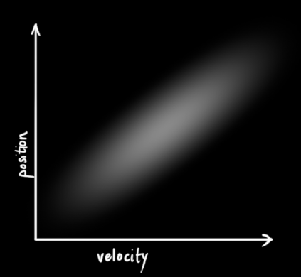
We don't know the actual positions and velocities, there are many possible correct combinations of them, but some are more likely than others:
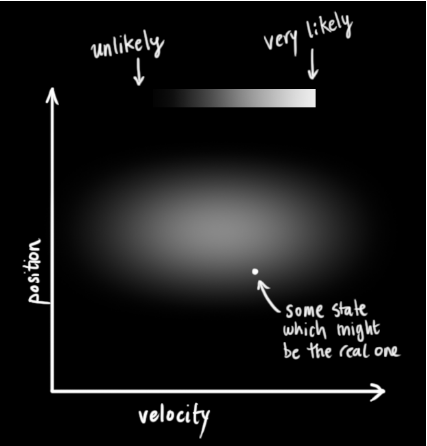
Kalman filtering assumes that both variables (position and velocity, in this example) are random and follow a Gaussian distribution. Each variable has a mean μ representing the center (most likely state) of the random distribution, and a variance
![]()
, representing uncertainty.
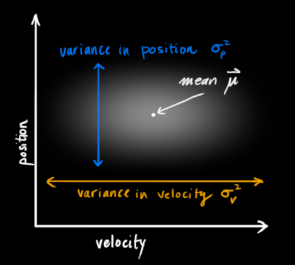
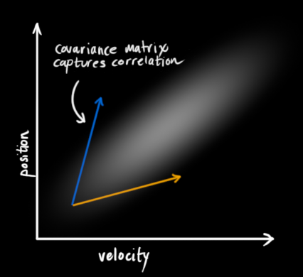
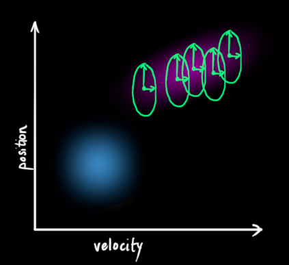
In the above diagram, position and velocity are uncorrelated, which means that the state of one variable cannot predict the possible value of the other variable. The following example is more interesting: position and velocity are related, and the probability of observing a particular position depends on the current velocity:
It is possible that, for example, we estimate a new position based on an old position. If the speed is too high, we may have moved very far. If you move slowly, the distance will not be very far. Tracking this relationship is very important because it brings us more information: one of the measured values tells us the possible values of other variables. Extract more information from your data!
This correlation is represented by a covariance matrix , in short, each element in the matrix
![]()
Indicates the degree of correlation between the i-th and j-th state variables. (You may have guessed that the covariance matrix is a symmetric matrix , which means that i and j can be swapped arbitrarily). The covariance matrix is usually represented by "
![]()
" to represent, and the elements in it are represented as "
![]()
”。
4. Use matrices to describe the problem
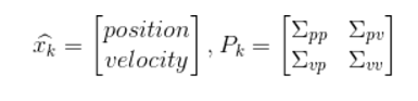
We build state variables based on a Gaussian distribution, so at time k we need two pieces of information: the best estimate
![]()
(that is, the mean value, commonly used elsewhere expressed as μ), and the covariance matrix
![]()
。
(1)
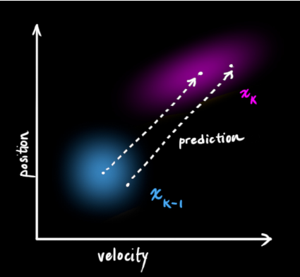
(Of course, here we only use position and velocity. In fact, this state can contain multiple variables, representing any information you want to represent). Next, we need to predict the next state (moment k) based on the current state (moment k-1). Remember, we don't know which of all the predictions for the next state is "true", but our prediction function doesn't care. It makes predictions for all possibilities and gives a new Gaussian distribution.
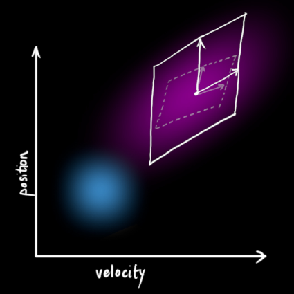
We can use the matrix
![]()
To represent this prediction process:
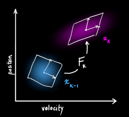
It moves each point in our original estimate to a new predicted location, which is where the system would move to next if the original estimate was correct. Then how do we use the matrix to predict the position and speed of the next moment? The following is expressed by a basic kinematics formula:
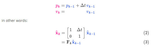
Now, we have a prediction matrix to represent the state at the next moment, however, we still don't know how to update the covariance matrix. At this point, we need to introduce another formula, if we multiply each point in the distribution by the matrix A, then its covariance matrix
![]()
How will it change? Very simple, the formula is given below:

Combining equations (4) and (3) yields:

5. External control volume
We have not captured all the information, and there may be external factors that will control the system and bring about some changes that are not related to the state of the system itself.
Taking the motion state model of a train as an example, the train driver may manipulate the accelerator to accelerate the train. Likewise, in our robot example, the navigation software might issue a command to turn the wheels or stop. Knowing this additional information, we can use a vector
![]()
to represent, and add it to our forecasting equation for correction.
Suppose we know the desired acceleration due to the setting of the throttle or the control command
![]()
, according to the basic kinematic equations:

In matrix form it is:
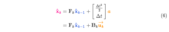
![]()
called the control matrix,
![]()
is called the control vector (for simple systems without external control, this part can be ignored). Let's think again, what if our predictions are not 100% accurate?
external interference
If these state quantities are changed based on the properties of the system itself or the known external control action, no problem will arise.
But what if there are unknown disturbances? For example, if we track a quadrotor, it might be disturbed by the wind, if we track a wheeled robot, the wheels might slip, or a small slope on the road slows it down . In this way, we cannot continue to track these states, and if these external disturbances are not taken into account, our predictions will be biased.
After each prediction, we can add some new uncertainty to model this uncertainty with the "outside world" (i.e. disturbances we are not tracking):
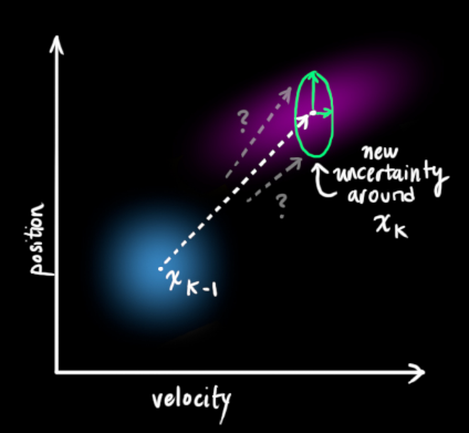
After each state variable in the original estimate is updated to a new state, it still obeys a Gaussian distribution. we can say
![]()
Each state variable of moves to a new Gaussian-distributed region with a covariance of
![]()
. In other words, we treat these untracked disturbances as having a covariance of
![]()
noise to deal with.
This produces a new Gaussian distribution with a different covariance (but the same mean).
We do this by simply adding
![]()
Obtaining the expanded covariance, the full expression for the prediction step is given below:
It can be seen from the above formula that the new optimal estimate is obtained based on the prediction of the previous optimal estimate , and the correction of the known external control quantity is added .
The new uncertainty is predicted by the previous uncertainty , and the external environment is added.
Well, we have a vague estimate of the likely behavior of the system, using
![]()
and
![]()
To represent. What happens if you combine the data from the sensors?
6. Use measurements to correct estimates
We may have multiple sensors to measure the current state of the system. It doesn't matter which sensor measures which state variable. Maybe one measures the position and the other measures the speed. Each sensor indirectly tells us some state information.
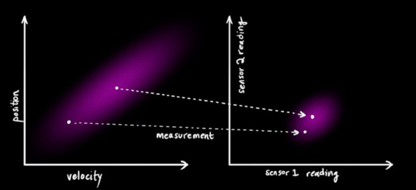
Note that the unit and scale of the data read by the sensor may be different from the unit and scale of the state we want to track. We use the matrix
![]()
to represent sensor data.
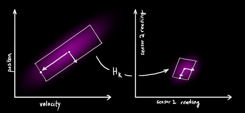
We can calculate the distribution of sensor readings, using the previous representation as follows:

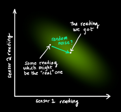
One of the great advantages of Kalman filtering is that it can handle sensor noise, in other words, our sensors are more or less unreliable, and each state in the raw estimate can correspond to a certain range of sensor readings.
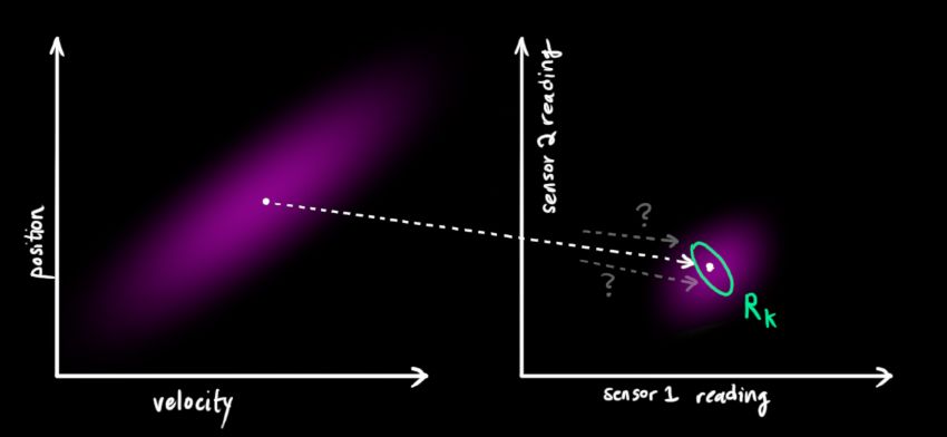
From the measured sensor data, we can roughly guess what state the system is currently in. But due to uncertainty, some states may be closer to the true state than the readings we get.
We use this uncertainty (eg: sensor noise) as the covariance
![]()
Indicates that the mean of the distribution is the sensor data we read, called
![]()
。
Now we have two Gaussian distributions, one around the predicted value and one around the sensor reading.
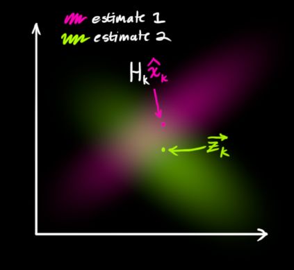
We have to find the optimal solution between predicted values (pink) and sensor measured values (green) .
So, what is our most likely state? For any possible reading
![]()
, there are two cases: (1) the measured value of the sensor; (2) the predicted value obtained from the previous state. If we want to know the probability that both of these situations can occur, multiplying these two Gaussian distributions will do the trick.
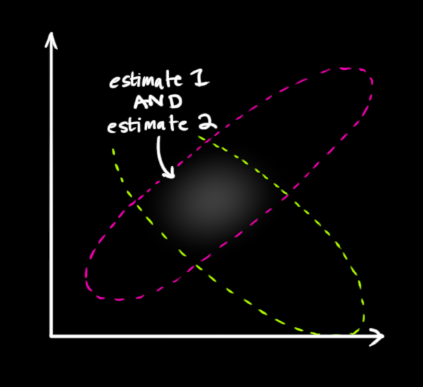
The rest is the overlap, and the mean of the overlap is the most likely value of the two estimates, that is, the best estimate given all the information.
Voila! This overlapping area looks like another Gaussian distribution.
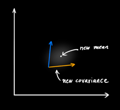
As you can see, by multiplying two Gaussian distributions with different means and variances, you get a new Gaussian distribution with independent means and variances! Explained below with the formula.
7. Fusion Gaussian distribution
First analyze the simpler points with a one-dimensional Gaussian distribution, with variance
![]()
The Gaussian curve of and μ can be expressed by the following formula:

What do you get if you multiply two Gaussian functions together?
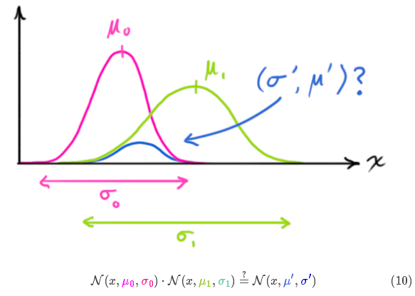
Substituting formula (9) into formula (10) (pay attention to renormalization, so that the total probability is 1) can get:

The same part of the two formulas in formula (11) is represented by k:

Next, formulas (12) and (13) are further written in matrix form, if Σ represents the covariance of Gaussian distribution,
![]()
represents the mean of each dimension, then:

matrix
![]()
It is called the Kalman gain and will be used below. Relax! We're almost done!
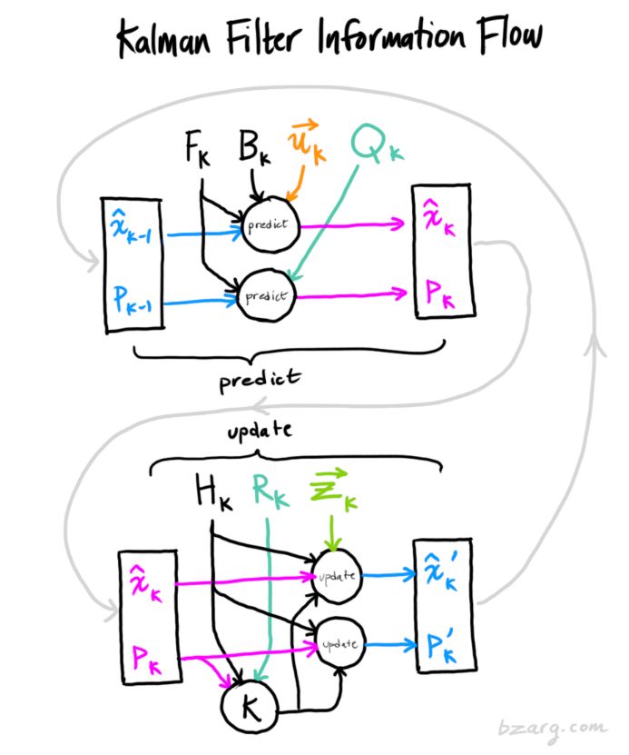
8. Put all the formulas together
We have two Gaussian distributions, the prediction part
![]()
, and the measurement section
![]()
, put them into formula (15) to calculate the overlap between them:

From equation (14), the Kalman gain can be obtained as:
![]()
Multiply both sides of formula (16) and formula (17) by the inverse of the matrix at the same time (note
![]()
which contains
![]()
) to reduce it, and then multiply both sides of the second equation of formula (16) to the right by the matrix at the same time
![]()
The inverse of gives the following equation:

The above formula gives the complete update step equation.
![]()
is the new optimal estimate, we can combine it with
![]()
Put it into the next prediction and update equation and iterate continuously.
Nine. Summary
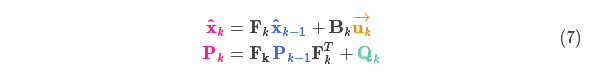
In all the above formulas, you only need to use formulas (7), (18), and (19). (If you forget, you can re-deduce it according to formulas (4) and (15))
We can use these formulas to establish an accurate model for any linear system. For nonlinear systems, we use extended Kalman filtering. The difference is that EKF has an additional process of linearizing the prediction and measurement parts.