6.2 Initial value of weight [Introduction to Deep Learning: Theory and Implementation Based on Python (Chapter 6 Skills Related to Learning)]
import numpy as np
import matplotlib.pyplot as plt
def sigmoid(x):
    return 1 / (1 + np.exp(-x))
vanishing gradient
x = np.random.randn(1000, 100) # 1000个数据,每个数据100个特征
hidden_layer_size =  5 # 5个隐藏层
node_num = 100 # 每个隐藏层100个节点
activations = {

    }

for i in range(hidden_layer_size):
    if i!=0:
        x = activations[i-1]

    w = np.random.randn(node_num, node_num) * 1
    z = np.dot(x, w)
    a = sigmoid(z)
    activations[i] = a
for i, a in activations.items():
    plt.subplot(1 ,len(activations), i+1)
    plt.title(str(i+1) + '-layer')
    plt.hist(a.flatten(), 30, range=(0,1))
plt.show()
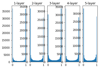
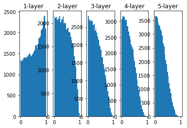
The activation values of each layer are distributed towards 0 and 1. The sigmoid function used here is an S-type function. As the output continues to approach 0 or 1, the value of its derivative becomes close to 0. Therefore, the data distribution biased towards 1 and 0 will cause the value of the gradient in backpropagation to change continuously. Small, and finally disappear, known as the vanishing gradient problem.
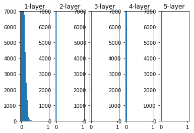
After changing the weights to a Gaussian distribution with a standard deviation of 0.01
limited expressiveness
x = np.random.randn(1000, 100) # 1000个数据,每个数据100个特征
hidden_layer_size =  5 # 5个隐藏层
node_num = 100 # 每个隐藏层100个节点
activations = {

    }

for i in range(hidden_layer_size):
    if i!=0:
        x = activations[i-1]

    w = np.random.randn(node_num, node_num) * 0.01
    z = np.dot(x, w)
    a = sigmoid(z)
    activations[i] = a
for i, a in activations.items():
    plt.subplot(1 ,len(activations), i+1)
    plt.title(str(i+1) + '-layer')
    plt.hist(a.flatten(), 30, range=(0,1))
plt.show()

This time the distribution of activation values is concentrated around 0.5. The problem of gradient disappearance will not occur, but the distribution of activation values is biased, which has a big problem in expressiveness. Why do you say that? Because if there are multiple neurons that are all outputting almost the same value, then there is no point for them to exist. For example, if 100 neurons are all outputting almost the same value, then 1 neuron can also say basically the same thing. Therefore, there is a problem of "limited expressiveness" when the activation value is biased in the distribution.
The distribution of the activation values of each layer requires an appropriate breadth. why? Because by passing diverse data between layers, neural networks can learn efficiently. Conversely, if biased data is passed, the problem of gradient disappearance or "limited expressiveness" will occur, and learning may not proceed smoothly.
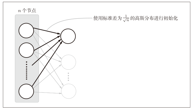
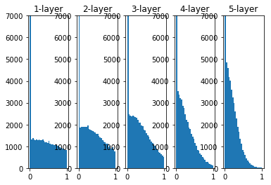
Xavier initial value
In order to make the activation values of each layer present a distribution with the same breadth, it is pushed to an appropriate weight scale. The deduced conclusion is that if the number of nodes in the previous layer is n, the initial value uses a standard deviation of 1 n \frac{1}{\sqrt{n}}n1Distribution
x = np.random.randn(1000, 100) # 1000个数据,每个数据100个特征
hidden_layer_size =  5 # 5个隐藏层
node_num = 100 # 每个隐藏层100个节点
activations = {

    }

for i in range(hidden_layer_size):
    if i!=0:
        x = activations[i-1]

    w = np.random.randn(node_num, node_num) / np.sqrt(node_num)
    z = np.dot(x, w)
    a = sigmoid(z)
    activations[i] = a
for i, a in activations.items():
    plt.subplot(1 ,len(activations), i+1)
    plt.title(str(i+1) + '-layer')
    # if i != 0: plt.yticks([], [])
    # plt.ylim(0, 6000)
    plt.hist(a.flatten(), 30, range=(0,1))
plt.show()
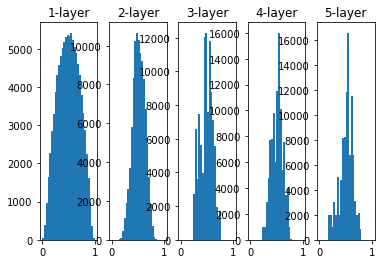
The further back the layers, the more skewed the image becomes, but more widely distributed than before. Since the data passed between layers has an appropriate breadth, the expressive power of the sigmoid function is not limited, and efficient learning is expected.
fishy
Replaced by tahn function, the shape is bell-shaped? The function used as the activation function preferably has the property of being symmetric about the origin
def tanh(x):
    return np.tanh(x)
x = np.random.randn(1000, 100) # 1000个数据,每个数据100个特征
hidden_layer_size =  5 # 5个隐藏层
node_num = 100 # 每个隐藏层100个节点
activations = {

    }

for i in range(hidden_layer_size):
    if i!=0:
        x = activations[i-1]

    w = np.random.randn(node_num, node_num) / np.sqrt(node_num)
    z = np.dot(x, w)
    a = tanh(z)
    activations[i] = a
for i, a in activations.items():
    plt.subplot(1 ,len(activations), i+1)
    plt.title(str(i+1) + '-layer')
    # if i != 0: plt.yticks([], [])
    # plt.ylim(0, 6000)
    plt.hist(a.flatten(), 30, range=(0,1))
plt.show()
The weight initial value of ReLU
The initial value of Xaiver is derived based on the activation function being a linear function. Because sigmoid and tanh are left and right symmetrical, and the vicinity of the center can be regarded as a linear function, it is suitable to use the initial value of Xaiver.
When the activation function uses ReLU, it is recommended to use the initial value dedicated to ReLU, called He initial value
When the number of nodes in the previous layer is n, the initial value of He uses a standard deviation of 2 n \sqrt{\frac{2}{n}}n2
When the initial value of Xaiver is 1 n \sqrt{\frac{1}{n}}n1When , it can be explained that because the value of the negative value area of ReLU is 0, in order to make it more extensive, it needs 2 times the coefficient
def ReLU(x):
    return np.maximum(0 ,x)
The initial value of the weight is a Gaussian distribution with a standard deviation of 0.01
x = np.random.randn(1000, 100) # 1000个数据,每个数据100个特征
hidden_layer_size =  5 # 5个隐藏层
node_num = 100 # 每个隐藏层100个节点
activations = {

    }

for i in range(hidden_layer_size):
    if i!=0:
        x = activations[i-1]

    w = np.random.randn(node_num, node_num) * 0.01
    z = np.dot(x, w)
    a = ReLU(z)
    activations[i] = a
for i, a in activations.items():
    plt.subplot(1 ,len(activations), i+1)
    plt.title(str(i+1) + '-layer')
    # if i != 0: plt.yticks([], [])
    # plt.xlim(0.1, 1)
    plt.ylim(0, 7000)
    plt.hist(a.flatten(), 30, range=(0,1))
plt.show()
When the weight initial value is the initial value of Xaiver
x = np.random.randn(1000, 100) # 1000个数据,每个数据100个特征
hidden_layer_size =  5 # 5个隐藏层
node_num = 100 # 每个隐藏层100个节点
activations = {

    }

for i in range(hidden_layer_size):
    if i!=0:
        x = activations[i-1]

    w = np.random.randn(node_num, node_num) * np.sqrt(1.0 / node_num)
    z = np.dot(x, w)
    a = ReLU(z)
    activations[i] = a
for i, a in activations.items():
    plt.subplot(1 ,len(activations), i+1)
    plt.title(str(i+1) + '-layer')
     # if i != 0: plt.yticks([], [])
    # plt.xlim(0.1, 1)
    plt.ylim(0, 7000)
    plt.hist(a.flatten(), 30, range=(0,1))
plt.show()
When the initial value of the weight is the initial value of He
x = np.random.randn(1000, 100) # 1000个数据,每个数据100个特征
hidden_layer_size =  5 # 5个隐藏层
node_num = 100 # 每个隐藏层100个节点
activations = {

    }

for i in range(hidden_layer_size):
    if i!=0:
        x = activations[i-1]

    w = np.random.randn(node_num, node_num) * np.sqrt(2.0 / node_num)
    z = np.dot(x, w)
    a = ReLU(z)
    activations[i] = a
for i, a in activations.items():
    plt.subplot(1 ,len(activations), i+1)
    plt.title(str(i+1) + '-layer')
    # if i != 0: plt.yticks([], [])
    plt.xlim(0.1, 1)
    plt.ylim(0, 7000)
    plt.hist(a.flatten(), 30, range=(0,1))
plt.show()

Summarize
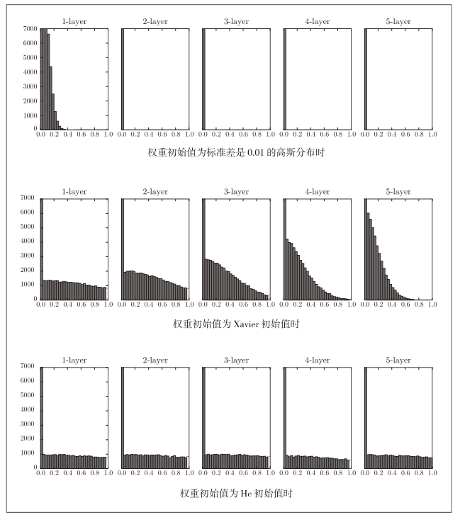
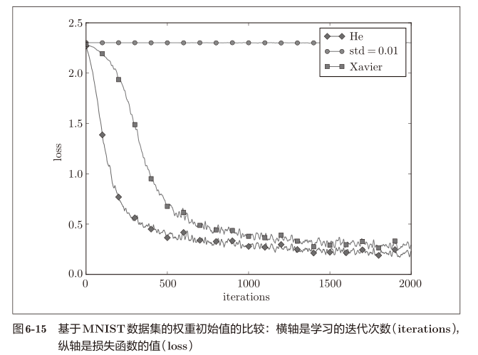
- When std=0.01, the activation value of each layer is very small, and the value transmitted on the neural network is also very small, indicating that the gradient of the weight during reverse propagation is also very small.
- When the initial value is Xaiver, as the number of layers deepens, the bias gradually becomes larger
- When the initial value is He, the breadth of the distribution in each layer is the same
Comparison of initial weight values based on MNIST dataset