[Introduction to Deep Learning: Theory and Implementation Based on Python]

perceptron

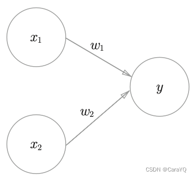
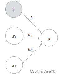
The perceptron receives multiple input signals and outputs a signal. The signal of the perceptron only has two values: "flow/no flow" (1/0). In this book, 0 corresponds to "no signal" and 1 corresponds to "signal". Figure 2-1 is an example of a perceptron that receives two input signals. x1, x2 are input signals, y is the output signal, w1, w2 are weights (w is the first letter of weight). The ○ in the figure is called a "neuron" or "node". When the input signal is sent to the neuron, it will be multiplied by a fixed weight (w1x1, w2x2) respectively. The neuron calculates the sum of the transmitted signals, and only outputs 1 when the sum exceeds a certain limit. This is also called "the neuron being activated". This limit is called the threshold here, represented by the symbol θ.

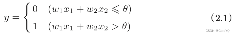
Expressing the above content in mathematical terms is equation (2.1):

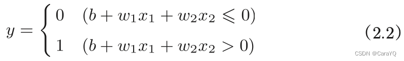
Replace θ in equation (2.1) with −b, and then equation (2.2) can be used to express the behavior of the perceptron.

Here −θ is named bias b. Note that the bias has different functions from weights w1 and w2. Specifically, w1 and w2 are parameters that control the importance of the input signal. The greater the weight, the higher the importance of the signal corresponding to that weight. The bias is a parameter that adjusts how easily a neuron is activated (the extent to which the output signal is 1).

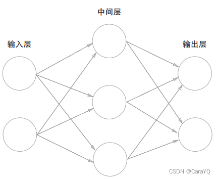
A perceptron with multiple layers superimposed is also called a multi-layer perceptron.
"Things that cannot be represented by a single-layer perceptron can be solved by adding another layer." In other words, by overlaying layers (deepening layers), the perceptron can be represented more flexibly.

Neural Networks

The disadvantage of the perceptron is that it requires manual setting to determine the appropriate weights that meet the expected input and output, while the neural network can automatically learn the appropriate weight parameters from the data.

From perceptron to neural network

Neural network example

This book agrees:

1. In Figure 3-1, layer 0 corresponds to the input layer, layer 1 corresponds to the middle layer, and layer 2 corresponds to the output layer. The
   network in Figure 3-1 is composed of 3 layers of neurons, but in fact only 2 layers of neurons have weights, so it is called a "2-layer network". Some books will also call the network in Figure 3-1 a three-layer network based on the number of layers that make up the network. In this book, the name of the network will
   be expressed according to the number of layers that actually have weights (the number of input layers, hidden layers, and output layers minus 1).

Review perceptron

The perceptron in Figure 3-2 receives three input signals x1, x2, and 1 and outputs y. b is a parameter called bias, used to control the ease with which neurons are activated; w1 and w2 are parameters representing the weight of each signal, used to control the importance of each signal. Expressed as a mathematical formula, it is shown in equation (3.1).

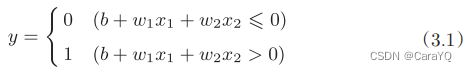
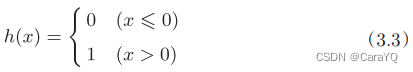
Figure 3-2 uses the three signals x1, x2, and 1 as inputs to the neuron. After multiplying them by their respective weights, they are sent to the next neuron. In the next neuron, the sum of these weighted signals is calculated. If this sum exceeds 0, output 1, otherwise output 0. We use a function to represent the action of this situation, introduce a new function h(x), and rewrite equation (3.1) into the following equation (3.2) and equation (3.3).

The activation function appears

The h(x) function just introduced will convert the sum of input signals into an output signal. This function is generally called an activation function and is used to determine how to activate the sum of input signals.
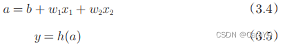
If Equation (3.2) is written in more detail, it can be divided into the following two equations:

If you want to express Equation (3.4) and Equation (3.5) clearly in the figure, you can do it like Figure 3-4.

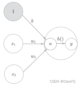
As shown in Figure 3-4, the calculation process of the activation function is clearly shown in ○ representing the neuron, that is, the weighted sum of the signals is neuron a, and then neuron a is converted into neuron y by the activation function h()

The activation function is the bridge between the perceptron and the neural network. When this book uses the term "perceptron", it does not strictly unify the algorithm it refers to. Generally speaking, "naive perceptron" refers to a single-layer network, which refers to a model whose activation function uses a step function A. "Multilayer perceptron" refers to a neural network, that is, a multilayer network using a smooth activation function such as the sigmoid function (described later).

activation function

The activation function represented by equation (3.3) is bounded by a threshold. Once the input exceeds the threshold, the output is switched. Such a function is called a "step function". Therefore, it can be said that the step function is used as the activation function in the perceptron. If you change the activation function from a step function to another function, you can enter the world of neural networks. Next we will introduce the activation function used by neural networks.

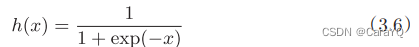
sigmoid function

An activation function often used in neural networks is the sigmoid function represented by equation (3.6)

Implementation of step function

The step function is shown in equation (3.3). When the input exceeds 0, it outputs 1, otherwise it outputs 0. A step function can be implemented simply like below.

def step_function(x):
 if x > 0:
 return 1
 else:
 return 0

In the above implementation, the parameter x can only accept real numbers (floating point numbers), and the parameter is not allowed to be a NumPy array. In order to facilitate subsequent operations, we modified it to support the implementation of NumPy arrays. We first prepared a NumPy array x and performed the inequality sign operation on this NumPy array.

>>> import numpy as np
>>> x = np.array([-1.0, 1.0, 2.0])
>>> x
array([-1., 1., 2.])
>>> y = x > 0
>>> y
array([False, True, True], dtype=bool)

After the inequality sign operation is performed on the NumPy array, each element of the array will be subjected to the inequality sign operation to generate a Boolean array. Here, elements greater than 0 in array x are converted to True, and elements less than or equal to 0 are converted to False, thereby generating a new array y.
The array y is a Boolean array, but the step function we want is a function that outputs an int type of 0 or 1. Therefore, it is necessary to convert the element type of array y from boolean to int.

>>> y = y.astype(np.int)
>>> y
array([0, 1, 1])

As shown above, you can convert the type of a NumPy array using the astype() method. The astype() method specifies the desired type through parameters, which is np.int in this example. After converting Boolean type to int type in Python, True will be converted to 1 and False will be converted to 0

Implementation of sigmoid function

def sigmoid(x):
 return 1 / (1 + np.exp(-x))

When the parameter x is a NumPy array, the result can also be calculated correctly. This is because of NumPy's broadcast function.

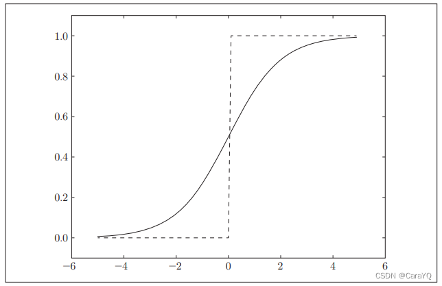
Comparison of sigmoid function and step function

Same point:

1. have similar shapes. In fact, the structure of both is "when the input is small, the output is close to 0 (is 0); as the input increases, the output is close to 1 (becomes 1)". That is to say, when the input signal is important information, both the step function and the sigmoid function will output a larger value; when the input signal is unimportant information, both will output a smaller value.
2. No matter how small or how big the input signal is, the value of the output signal is between 0 and 1
3. Both are nonlinear functions.

The activation function of the neural network must use a nonlinear function. Because if you use a linear function, it makes no sense to deepen the number of layers of the neural network. The problem with linear functions is that no matter how deep the layers are, there is always an equivalent "neural network without hidden layers".

difference:

1. The difference in "smoothness". The sigmoid function is a smooth curve, and the output changes continuously with the input. The step function is bounded by 0, and the output changes drastically.
2. Compared with the step function which can only return 0 or 1, the sigmoid function can return real numbers such as 0.731..., 0.880... (this is related to the smoothness just mentioned). In other words, what flows between the neurons in the perceptron is a binary signal of 0 or 1, while what flows in the neural network is a continuous real-valued signal.

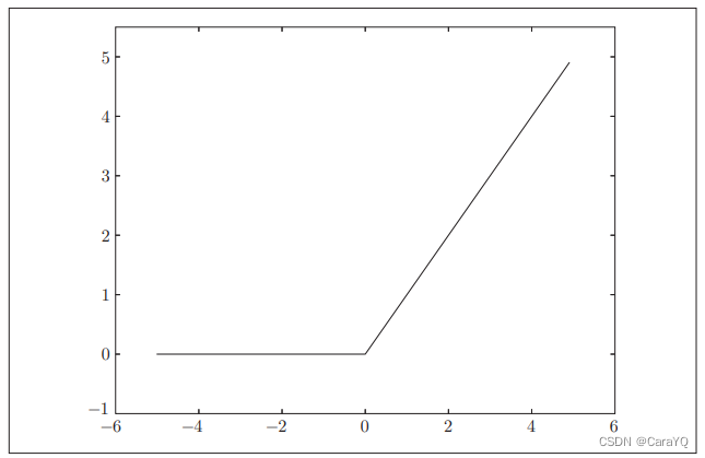
ReLU function

In the history of the development of neural networks, the sigmoid function has been used very early, and recently the ReLU (Rectified Linear Unit) function has been mainly used. When the input is greater than 0, the ReLU function directly outputs the value; when the input is less than or equal to 0, it outputs
0 (Figure 3-9). The ReLU function can be expressed as the following formula (3.7).


Implementation of ReLU function:

def relu(x):
 return np.maximum(0, x)

Implementation of 3-layer neural network

Symbol confirmation

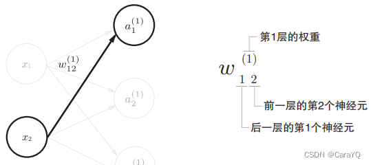
There is a "(1)" in the upper right corner of the weight and hidden layer neurons, which indicates the weight and layer number of the neuron (ie, the weight of layer 1, the neuron of layer 1). In addition, there are two numbers in the lower right corner of the weight, which are the index numbers of the neurons in the next layer and the neurons in the previous layer.

Code

# 保存每一层所需的参数（权重和偏置）
def init_network():
 network = {
    
    }
 network['W1'] = np.array([[0.1, 0.3, 0.5], [0.2, 0.4, 0.6]])
 network['b1'] = np.array([0.1, 0.2, 0.3])
 network['W2'] = np.array([[0.1, 0.4], [0.2, 0.5], [0.3, 0.6]])
 network['b2'] = np.array([0.1, 0.2])
 network['W3'] = np.array([[0.1, 0.3], [0.2, 0.4]])
network['b3'] = np.array([0.1, 0.2])
 return network
def forward(network, x):
 W1, W2, W3 = network['W1'], network['W2'], network['W3']
 b1, b2, b3 = network['b1'], network['b2'], network['b3']
 a1 = np.dot(x, W1) + b1
 z1 = sigmoid(a1)
 a2 = np.dot(z1, W2) + b2
 z2 = sigmoid(a2)
 a3 = np.dot(z2, W3) + b3
 y = identity_function(a3)
 return y
network = init_network()
x = np.array([1.0, 0.5])
y = forward(network, x)
print(y) # [ 0.31682708 0.69627909]

Output layer design

Neural networks can be used in classification problems and regression problems, but the activation function of the output layer needs to be changed according to the situation. Generally speaking, the identity function is used for regression problems and the softmax function is used for classification problems.

Machine learning problems can be roughly divided into classification problems and regression problems. Classification problem is the question of which category the data belongs to. For example, the problem of distinguishing whether a person in an image is male or female is a classification problem. The regression problem is the problem of predicting a (continuous) numerical value based on some input. For example, the problem of predicting a person's weight based on an image is a regression problem (prediction like "57.4kg")

Identity function and softmax function

The identity function will output the input as it is, and the input information will be output directly without any modification.
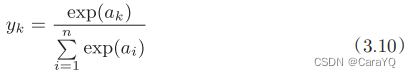
The softmax function used in classification problems can be expressed by the following formula (3.10), and its output can be understood as "probability"

to implement the softmax function

>>> a = np.array([0.3, 2.9, 4.0])
>>>
>>> exp_a = np.exp(a) # 指数函数
>>> print(exp_a)
[ 1.34985881 18.17414537 54.59815003]
>>>
>>> sum_exp_a = np.sum(exp_a) # 指数函数的和
>>> print(sum_exp_a)
74.1221542102
>>>
>>> y = exp_a / sum_exp_a
>>> print(y)
[ 0.01821127 0.24519181 0.73659691]

Although the above implementation correctly describes equation (3.10), overflow problems may occur in computer operations. The implementation of the softmax function requires the calculation of the exponential function, but at this time the value of the exponential function can easily become very large. For example, the value of e10 will exceed 20,000, e100 will become a very large value followed by more than 40 zeros, and the result of e1000 will return an inf indicating infinity. If you divide between these very large values, the result will be "indeterminate". Based on this, we make the following improvements:

First, multiply both the numerator and denominator of equation (3.11) by C, an arbitrary constant. Then, move this C into the exponential function (exp) and record it as log C. Finally, replace log C with another symbol C'. Equation (3.11) shows that when performing the calculation of the softmax exponential function, adding (or subtracting) a certain constant will not change the result of the calculation. C' here can use any value, but in order to prevent overflow, the maximum value in the input signal is generally used. To sum up, we can implement the softmax function as follows.

def softmax(a):
 c = np.max(a)
 exp_a = np.exp(a - c) # 溢出对策
 sum_exp_a = np.sum(exp_a)
 y = exp_a / sum_exp_a
 return y

Generally speaking, neural networks only use the category corresponding to the neuron with the largest output value as the recognition result. Moreover, even if the softmax function is used, the position of the neuron with the largest output value will not change. Therefore, when the neural network performs classification, the softmax function of the output layer can be omitted. In actual problems, since the operation of the exponential function requires a certain amount of computer operations, the softmax function of the output layer is generally omitted.

The steps to solve machine learning problems can be divided into two stages: "learning" and "inference". First, the model is learned B in the learning phase, and then, in the inference phase, the learned model is used to infer (classify) unknown data. As mentioned before, the softmax function of the output layer is generally omitted in the inference stage. The softmax function is used in the output layer because it is related to the learning of neural networks.

Number of neurons in the output layer

For classification problems, the number of neurons in the output layer is generally set to the number of categories.

Handwritten digit recognition

Just like the steps for solving machine learning problems (divided into two stages: learning and inference), when using neural networks to solve problems, you also need to first use training data (learning data) to learn weight parameters; when performing inference, use the just-learned parameters, classify the input data, and the inference process is also called the forward propagation of the neural network

MNIST dataset

The general method of using the MNIST data set is to first use training images to learn, and then use the learned model to measure the extent to which test images can be correctly classified. The image data of MNIST is a 28 pixel × 28 pixel grayscale image (1 channel), and
the value of each pixel is between 0 and 255. Each image data is marked with labels such as "7", "2", and "1" accordingly.
This book provides a convenient Python script mnist.py, which supports processing from downloading the MNIST data set to converting these data into NumPy arrays (mnist.py is in the dataset directory), using the load_mnist() function in mnist.py , you can easily read in MNIST data as follows.

import sys, os
sys.path.append(os.pardir) # 为了导入父目录中的文件而进行的设定
from dataset.mnist import load_mnist
# 第一次调用会花费几分钟 ……
(x_train, t_train), (x_test, t_test) = load_mnist(flatten=True,
normalize=False)
# 输出各个数据的形状
print(x_train.shape) # (60000, 784)
print(t_train.shape) # (60000,)
print(x_test.shape) # (10000, 784)
print(t_test.shape) # (10000,)

The above code is in the mnist_show.py file. The current directory of the mnist_show.py file is ch03, but the mnist.py file containing the load_mnist() function is in the dataset directory. Therefore, the mnist_show.py file cannot directly import the mnist.py file across directories. The sys.path.append(os.pardir) statement actually adds the parent directory deep-learning-from-scratch to sys.path (the path set of Python’s search module), so that deep-learning-from-scratch can be imported Any file in any directory (including the dataset directory)
under the load_mnist function returns the read MNIST data in the form of "(training image, training label), (test image, test label)". In addition, you can also set 3 parameters like load_mnist(normalize=True, flatten=True, one_hot_label=False). The first parameter normalize sets whether to normalize the input image to a value between 0.0 and 1.0. If this parameter is set to False, the pixels of the input image will remain the original 0 to 255. The second parameter flatten sets whether to expand the input image (into a one-dimensional array). If this parameter is set to False, the input image will be a three-dimensional array of 1 × 28 × 28; if set to True, the input image will be saved as a one-dimensional array composed of 784 elements. The third parameter one_hot_label sets whether to save the label as one-hot representation. One-hot means that only the array whose label is 1 is correctly solved, and the rest are all 0, just like [0,0,1,0,0,0,0,0,0,0]. When one_hot_label is False, the correct solution label is simply saved like 7 and 2; when one_hot_label is True, the label is saved as one-hot representation

Python has the convenient function of pickle. This function can save objects in the running program as files. If you load a saved pickle file, you can immediately restore the objects in the previous program run. The load_mnist() function used to read the MNIST data set also uses the pickle function internally (when reading for the second time and subsequent times). Using the pickle function, the preparation of MNIST data can be completed efficiently.

Display an MNIST image (source code is in ch03/mnist_show.py)

import sys, os
sys.path.append(os.pardir)
import numpy as np
from dataset.mnist import load_mnist
from PIL import Image
def img_show(img):
 pil_img = Image.fromarray(np.uint8(img))
 pil_img.show()
(x_train, t_train), (x_test, t_test) = load_mnist(flatten=True,
normalize=False)
img = x_train[0]
label = t_train[0]
print(label) # 5
print(img.shape) # (784,)
img = img.reshape(28, 28) # 把图像的形状变成原来的尺寸
print(img.shape) # (28, 28)
img_show(img)

It should be noted here that the image read when flatten=True is saved in the form of a column (one-dimensional) NumPy array. Therefore, when displaying the image, it needs to be changed to its original shape of 28 pixels × 28 pixels. You can change the shape of a NumPy array by specifying the desired shape as an argument to the reshape() method. In addition, the image data saved as a NumPy array also needs to be converted into a data object for PIL. This conversion process is completed by Image.fromarray().

Neural network inference processing

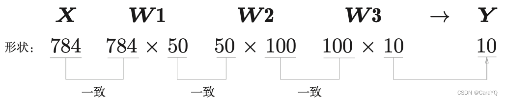
The input layer of the neural network has 784 neurons and the output layer has 10 neurons. The number 784 in the input layer comes from the image size of 28 × 28 = 784, and the number 10 in the output layer comes from the 10 category classification (numbers 0 to 9, 10 categories in total). In addition, this neural network has 2 hidden layers, the first hidden layer has 50 neurons and the second hidden layer has 100 neurons. The 50 and 100 can be set to any value. Next, we first define three functions: get_data(), init_network(), and predict() (the code is in ch03/neuralnet_mnist.py).

def get_data():
	(x_train, t_train), (x_test, t_test) = load_mnist(normalize=True, flatten=True, one_hot_label=False) 
	return x_test, t_test

# init_network()会读入保存在pickle文件sample_weight.pkl中的学习到的权重参数A。这个文件中以字典变量的形式保存了权重和偏置参数
def init_network():
	with open("sample_weight.pkl", 'rb') as f:
		network = pickle.load(f) 
	return network

def predict(network, x):
	W1, W2, W3 = network['W1'], network['W2'], network['W3'] 
	b1, b2, b3 = network['b1'], network['b2'], network['b3']
	a1 = np.dot(x, W1) + b1 z1 = sigmoid(a1)
	a2 = np.dot(z1, W2) + b2 z2 = sigmoid(a2)
	a3 = np.dot(z2, W3) + b3 y = softmax(a3)
	return y

First obtain the MNIST data set and generate a network. Then, use the for statement to retrieve the image data stored in x one by one, and use the predict() function for classification. The predict() function outputs the probability corresponding to each label in the form of a NumPy array. For example, if an array of [0.1, 0.3, 0.2, …, 0.04] is output, the array indicates that the probability of "0" is 0.1, the probability of "1" is 0.3, and so on. Then, we take out the index of the maximum value in this probability list (which element has the highest probability) as the prediction result. You can use the np.argmax(x) function to get the index of the maximum value in the array. np.argmax(x) will get the index of the maximum value element in the array assigned to parameter x. Finally, the answer predicted by the neural network is compared with the correct solution label, and the probability of the correct answer is taken as the recognition accuracy.

x, t = get_data() network = init_network()

accuracy_cnt = 0
for i in range(len(x)):
	y = predict(network, x[i])
	p = np.argmax(y) # 获取概率最高的元素的索引 
	if p == t[i]:
		accuracy_cnt += 1
		
print("Accuracy:" + str(float(accuracy_cnt) / len(x)))

After executing the above code, "Accuracy:0.9352" will be displayed. This means that 93.52% of the data is correctly classified

In this example, we set the parameter normalize of the load_mnist function to True. After normalize is set to True, the function will perform conversion internally, dividing each pixel value of the image by 255, so that the value of the data is in the range of 0.0~1.0. The process of limiting data to a certain range like this is called normalization. In addition, performing a certain transformation on the input data of the neural network is called pre-processing. Here, as a preprocessing of the input image, we perform regularization.
In fact, a lot of preprocessing takes into account the overall distribution of the data. For example, use the mean or standard deviation of the entire data to move the data so that the entire data is distributed around 0, or normalize it to control the extension of the data within a certain range. In addition, there are methods of uniformizing the distribution shape of the entire data, namely data whitening, etc.

Batch processing

Use the Python interpreter to output the shape of the weights of each layer of the neural network just now.

>>> x, _ = get_data()
>>> network = init_network()
>>> W1, W2, W3 = network['W1'], network['W2'], network['W3'] 
>>>
>>> x.shape (10000, 784) >>> x[0].shape (784,)
>>> W1.shape
(784, 50) 
>>> W2.shape 
(50, 100) 
>>> W3.shape 
(100, 10)

As shown in Figure 3-26, after inputting a one-dimensional array consisting of 784 elements (originally a 28 × 28 two-dimensional array), it outputs a one-dimensional array with 10 elements. This is the processing flow when only one image data is input.

Now let's consider the case of packaging and inputting multiple images. For example, we want to use the predict() function to package and process 100 images at one time. To do this, you can change the shape of x to 100 × 784 and pack 100 images as input data. If represented by a diagram, it is shown in Figure 3-27.

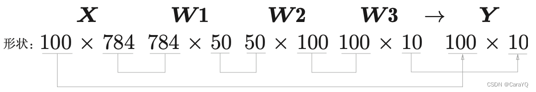
As shown in Figure 3-27, the input data has a shape of 100 × 784, and the output data has a shape of 100 × 10. This means that the results of the input 100 images are output at once. For example, x[0] and y[0] store the 0th image and its inference results.

This packaged input data is called a batch.

Below we implement batch-based code implementation:

x, t = get_data() 
network = init_network()

batch_size = 100 # 批数量 
accuracy_cnt = 0

for i in range(0, len(x), batch_size):
	x_batch = x[i:i+batch_size]
	y_batch = predict(network, x_batch)
	p = np.argmax(y_batch, axis=1)
	accuracy_cnt += np.sum(p == t[i:i+batch_size])

print("Accuracy:" + str(float(accuracy_cnt) / len(x)))

If the range() function is specified as range(start, end), it will generate a list consisting of integers between start and end-1. If you specify 3 integers like range(start, end, step), the next element in the generated list will be increased by the value specified by step. Let's look at an example.

>>> list( range(0, 10) )
[0, 1, 2, 3, 4, 5, 6, 7, 8, 9]

>>> list( range(0, 10, 3) )
[0, 3, 6, 9]

Based on the list generated by the range() function, batch data is extracted from the input data via x[i:i+batch_size]. x[i:i+batch_n] will take out the data from the i-th to the i+batch_n-th.
Then, get the index of the element with the largest value through argmax(). It should be noted that we have given the parameter axis=1. This specifies the index A of the element with the largest value found along the 1st dimension (with the 1st dimension as the axis) in a 100×10 array (the 0th dimension corresponds to the 1st dimension). Let’s also look at an example here.

>>> x = np.array([[0.1, 0.8, 0.1], [0.3, 0.1, 0.6], ... [0.2, 0.5, 0.3], [0.8, 0.1, 0.1]])
>>> y = np.argmax(x, axis=1)
>>> print(y)
[1 2 1 ... 0]

The 0th dimension of the matrix is ​​the column direction, and the 1st dimension is the row direction.

Finally, we compare the batch-wise classification results with the actual answers. To do this, you need to use the comparison operator (==) between NumPy arrays to generate a Boolean array composed of True/False, and count the number of True. We confirm this with the example below.

>>> y = np.array([1, 2, 1, 0]) 
>>> t = np.array([1, 2, 0, 0]) 
>>> print(y==t)
[True True False True]
>>> np.sum(y==t) 3

Neural network learning

The characteristic of neural networks is that they can learn from data. The so-called "learning from data" means that the values ​​of weight parameters can be automatically determined from the data.

With a finite number of learnings, linearly separable problems are solvable. However, nonlinear separable problems cannot be solved by (automatic) learning

Learn from data

Features are first extracted from the image, and then machine learning technology is used to learn the patterns of these features. The "feature quantity" mentioned here refers to
a converter that can accurately extract essential data (important data) from input data (input image). The feature quantities of images are usually expressed in the form of vectors

Whether the problem to be solved is to identify 5, dogs, or faces, neural networks try to find patterns in the problem to be solved by continuously learning the data provided.

training data and test data

In machine learning, data is generally divided into two parts: training data and test data for learning and experiments. First, use training data to learn and find optimal parameters; then, use test data to evaluate the actual capabilities of the trained model. Why do we need to divide the data into training data and test data? Because what we are pursuing is the generalization ability of the model. In order to correctly evaluate the generalization ability of the model, it is necessary to divide the training data and test data. In addition, training data can also be called supervised data. Generalization ability refers to the ability to process unobserved data (data not included in the training data). Achieving generalization capabilities is the ultimate goal of machine learning.

The state of overfitting only a certain data set is called overfitting.

loss function

The learning of the neural network represents the current state through a certain indicator, that is, the neural network uses a certain indicator as a clue to find the optimal weight parameters. The indicator used in the learning of neural networks is called the loss function. This loss function can use any function, but generally the mean square error and cross-entropy error are used.
The loss function is an indicator of the "badness" of the neural network's performance, that is, the extent to which the current neural network does not fit the supervised data and is inconsistent.

mean square error

The most famous loss function is the mean square error:

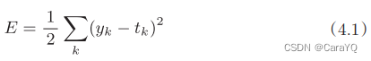
yk represents the output of the neural network, tk represents the supervised data, and k represents the dimensionality of the data. For example, in the example of handwritten digit recognition in Section 3.6, yk and tk are data composed of the following 10 elements.

>>> y = [0.1, 0.05, 0.6, 0.0, 0.05, 0.1, 0.0, 0.1, 0.0, 0.0]
>>> t = [0, 0, 1, 0, 0, 0, 0, 0, 0, 0]

The indexes of the array elements correspond to the numbers "0", "1", "2" starting from the first... Here, the output y of the neural network is the output of the softmax function. Since the output of the softmax function can be understood as probability, the above example indicates that the probability of "0" is 0.1, the probability of "1" is 0.05, the probability of "2" is 0.6, etc. t is supervised data, the correct solution label is set to 1, and the others are set to 0. Here, the label "2" is 1, indicating that the correct solution is "2". The representation method that represents the correct solution label as 1 and other labels as 0 is called one-hot representation.