Hello everyone, I recently learned the CS231N Stanford Computer Vision Open Class. It was so wonderful that I would like to share it with you.

1. Weight initialization

1.1 The same initialization weights

All weights in a neural network can be optimized and updated through gradient descent and backpropagation. Now the question is, what happens if the weights of each layer are all initialized to the same constant, and the constants of different layers can be different .

This will cause all neurons in the same layer to forward and back propagate exactly the same .

As shown in the figure below, in the process of forward propagation, the input received by each hidden layer is the same (x1, x2,...), and the weight of each hidden layer neuron corresponding to each input neuron is the same , then The output of each hidden layer neuron is the same. Then their back-propagated gradients must be the same .

It is equivalent to only one node in the hidden layer, and the input and output of other hidden layer neurons are the same as it. Even if there are 500 neurons, only one neuron's feature can be learned , which is different from having only one neuron. no difference.

Therefore, a multi-layer neural network cannot initialize the weights to the same number, otherwise the symmetry cannot be broken.

1.2 Too small initialization weights

Now randomly initialize each weight, such as using numpy's random standard normal distribution (mean=0, variance=1), as follows, Din represents the number of neurons in the previous layer, and Dout represents the number of neurons in this layer . Multiply by 0.01 for magnitude scaling.

# 生产Din行Dout列的矩阵，每个元素都服从标准正态分布
w = 0.01 * np.random.randn(Din, Dout)

Now using a 6-layer neural network, each layer has 4096 neurons, using the hyperbolic tangent tanh activation function (output is between -1 and 1), the output distribution of each layer is represented by a histogram. As shown in the figure below, we find that the further to the back layer, the closer the output of the neuron is to 0, and the standard deviation is getting smaller and smaller and closer to 0

The output of each neuron: $f(\sum_{i}w_{i}x_{i}+b)$ , f represents the activation function.

Find the partial derivative of Wi: $\frac{\partial f}{\partial w_{i}}=f'\times x_{i}$ , xi represents the output of the neuron in the previous layer. Since the output of the neuron is getting closer and closer to 0, the partial derivative is very close to 0, and the gradient disappears at this time.

It is precisely because of the smaller weight initialization that as the number of layers deepens, the output value of each neuron gets closer and closer to 0, and all values are concentrated around 0. Then after the partial derivative is calculated, xi tends to 0, and the gradient will be equal to 0, the gradient disappears

1.3 Oversized weight initialization

That is now initialized with larger weights . Multiply by 0.05 for magnitude scaling . what will happen

# 生产Din行Dout列的矩阵，每个元素都服从标准正态分布
w = 0.05 * np.random.randn(Din, Dout)

Using the same network structure as above, now using a 6-layer neural network with 4096 neurons in each layer, using the hyperbolic tangent tanh activation function (output between -1 and 1), using a histogram to represent the output distribution. As shown in the figure below, the output of each layer is concentrated in the saturation region (the hyperbolic tangent has a saturation region of -1 and 1)

The output of each neuron: $f(\sum_{i}w_{i}x_{i}+b)$ , f represents the hyperbolic tangent activation function.

Find the partial derivative with respect to Wi: $\frac{\partial f}{\partial w_{i}}=f'\times x_{i}$ , xi represents the output of the neuron in the previous layer, and the output of the neuron is getting closer and closer to -1 and 1; $f'$ it represents the derivative of the hyperbolic tangent function. Since the curve values are all in the saturation region at this time, the derivative is very close to 0, the gradient disappears at this time.

1.4 Xavier initialization method

In order to avoid problems caused by too large or too small initialization weights, the Xaviver initialization method determines the initialization weights according to the input dimension , and puts the square root of the input dimension on the denominator as a penalty. If the input dimension is large, the denominator is large, the weight initialization is relatively small, and the magnitude of the weight is adjusted adaptively .

In the convolutional neural network, Din represents the size of the receptive field, Din=kernel_size^2 * input_channels

As shown in the figure below, the output of each layer is neither concentrated in the saturation region nor near 0, and is evenly distributed in the interval from -1 to 1. And as the number of layers deepens, the input and output of each layer are very similar.

The more dimensions of the input, the more complex and variable the input is, and a larger penalty needs to be given, and the smaller the magnitude of the weight initialization is.

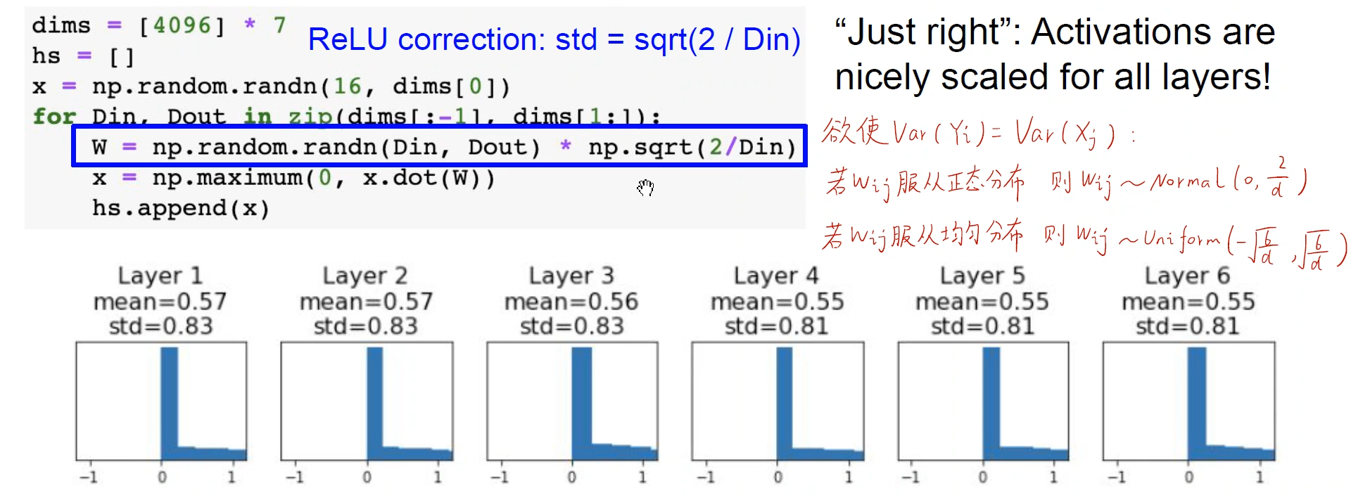
1.5 Kaiming initialization method

Since the Xavier initialization assumes that w and x are symmetric about 0, and the Xavier initialization method does not consider the activation function . However, the Xavier method does not hold in the ReLU method, because the output results of the ReLU activation function are all greater than or equal to 0. If Xavier is initialized in ReLU, the output of each layer of the neural network will be concentrated around 0, and the gradient will disappear.

He Kaiming used the Kaiming initialization method in ResNet to solve the above problems.

(1) The Kaiming initialization method uses the Xavier initialization method under the condition that the output is symmetrical about 0

(2) Different weights are explored. If you want the variance of input and output to be the same , ① If Wij obeys a normal distribution, the weights need to satisfy a normal distribution with 0 as the mean and d/2 as the standard deviation; ② If Wij obeys a uniform distribution, the weights need to obey $-\sqrt{\frac{6}{d}}$ the uniform distribution $\sqrt{\frac{6}{d}}$ between distributed

As shown in the figure below, the output results of each layer will not be limited to a particularly small area or saturated area in the positive value area.

2. Batch Normalization

2.1 Training Phase

Now we want the intermediate results of the neural network layer to follow a standard normal distribution , and we don't want the output values to all cluster to 0 or all in the saturation region. Forcing the output of the intermediate layer to undergo standard normal distribution transformation is Batch Normalization

Now there are N data in a batch, and each data is D-dimensional (D features). Equivalent to a matrix with N rows and D columns. Now take the mean of each column and find the D means. That is, to find the mean of a certain column of each data in the N data of a batch, that is, the mean of all the data in a certain column $\mu j$ . Then find the variance of all the data on a certain column $\sigma_{j}^{2}$ . Finally, batch normalization is performed on each data in the batch . where $\varepsilon$ is a very small number, make sure the denominator is not 0

Sometimes it is not good to forcibly convert to a standard normal distribution, so two parameters, $\gamma ,\beta$ , are introduced, which need to be learned in the network to optimize the batch normalization results above.

The final output is: $y_{i,j} = \gamma _{j}\hat{x}_{i,j}+\beta _{j}$

The role of Batch Normalization in the training phase is to pull the output results of the intermediate layer as far as possible, so that the gradient is exposed as much as possible.

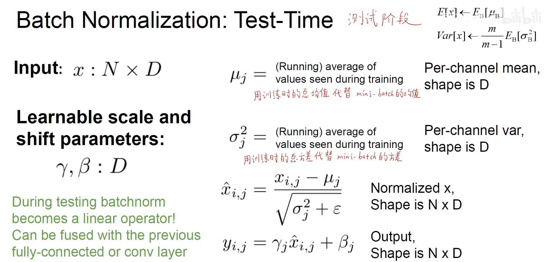
2.2 Test phase

The test phase is to test one data one by one, batch_size=1, there is no N data. Therefore, in the training process, it is necessary to save the mean and standard deviation of each batch of data, and finally obtain a global mean and standard deviation . In the testing phase, the global mean and standard deviation obtained in the training phase are used for Batch Normalization

The mean and variance of each batch are replaced by the total mean and total variance during training, and other steps are the same as in the training phase.

2.3 Use in Convolutional Neural Networks

In a fully connected neural network, there are N data in a batch, and each data is D-dimensional, and D means and variances are obtained. Learning in the network $\gamma ,\beta$ (each with D), the final batch normalized result is: $y = \gamma (x-\mu )/\sigma +\beta$ . These two parameters are used separately after each dimension is normalized separately.

In a convolutional neural network , there are N pieces of data in a batch, and each image uses C convolution kernels to generate C feature maps, and the length and width of each feature map are H * W respectively. For each channel, the mean and standard deviation of the entire batch are obtained, and C means and C standard deviations are obtained, and then each channel is trained separately $\gamma , \beta$ . These two parameters are used individually after each channel is normalized individually.

The role of Batch Normalization

Speed up convergence; improve gradients (away from saturation region); use large learning rates to avoid gradient disappearance; insensitive to initialization; regularizers.

[Deep Learning Theory] (4) Weight initialization, Batch Normalization