basic concept
overview
Autoencoder is an unsupervised learning neural network model for learning low-dimensional representation of data. It consists of two parts: an encoder (Encoder) and a decoder (Decoder). By compressing the input data into a low-dimensional encoding space, the input data is reconstructed from the encoding space.
basic structure
The basic structure of an autoencoder is as follows:
1. Encoder: Receives input data and maps it to a low-dimensional encoding space. The encoder consists of a sequence of hidden layers, usually with progressive dimensionality reduction for feature extraction and data compression.
2. Decoder (Decoder): Receives the output of the encoder and maps the encoded data back to the original input space. The structure of the decoder is the opposite of the encoder, gradually increasing the dimensionality and trying to reconstruct the original data.
3. Reconstruction Loss: The goal of an autoencoder is to reconstruct the input data as accurately as possible. Therefore, a reconstruction loss function is used to measure the difference between the original data and the reconstructed data, such as mean squared error (MSE) or cross-entropy loss.
training process
1. Provide the input data to the encoder to obtain a low-dimensional encoding.
2. Pass the encoded result to the decoder to try to reconstruct the input data.
3. Calculate the reconstruction loss, and optimize the network parameters through backpropagation to minimize the reconstruction error.
Repeat the above steps until the autoencoder can accurately reconstruct the input data.
application
1. Data dimensionality reduction: Autoencoders can learn low-dimensional representations of data, which is helpful for data compression and dimensionality reduction.
2. Feature learning: By training the autoencoder, meaningful feature representations of the data can be learned for subsequent supervised learning tasks.
3. Anomaly detection: Autoencoders can learn the normal distribution of data, which can be used to detect anomalies or reconstruction errors of anomalous data.
Detailed code and comments
import torch
import torch.nn as nn
import torch.utils.data as Data
import torchvision
import matplotlib.pyplot as plt
from mpl_toolkits.mplot3d import Axes3D
from matplotlib import cm
import numpy as np
# torch.manual_seed(1) # reproducible
# Hyper Parameters
EPOCH = 10
BATCH_SIZE = 64
LR = 0.005 # learning rate
DOWNLOAD_MNIST = True
N_TEST_IMG = 5
# Mnist digits dataset
train_data = torchvision.datasets.MNIST(
root='./mnist/',
train=True, # this is training data
transform=torchvision.transforms.ToTensor(), # Converts a PIL.Image or numpy.ndarray to
# torch.FloatTensor of shape (C x H x W) and normalize in the range [0.0, 1.0]
download=DOWNLOAD_MNIST, # download it if you don't have it
)
# plot one example
# 训练数据
print(train_data.train_data.size()) # (60000, 28, 28)
# 训练标签
print(train_data.train_labels.size()) # (60000)
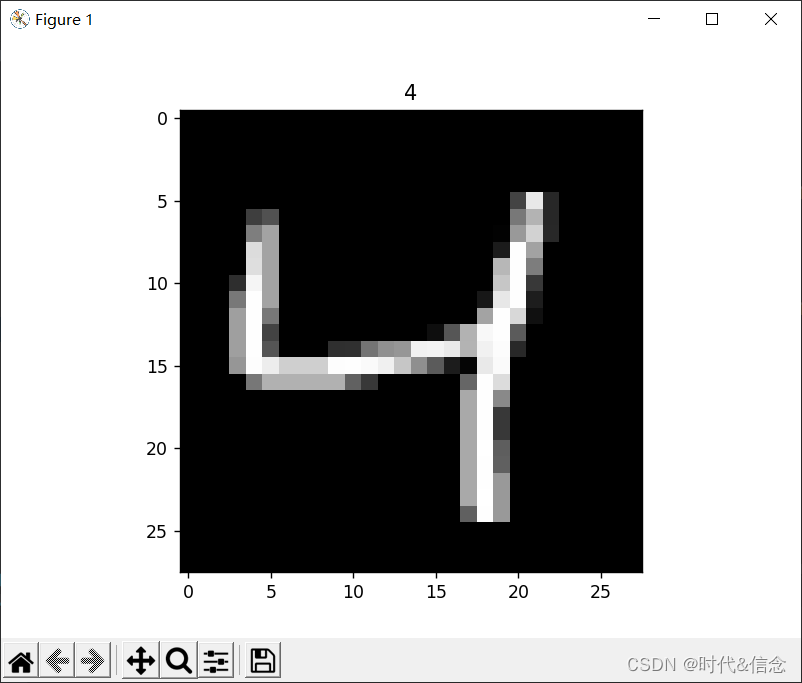
plt.imshow(train_data.train_data[2].numpy(), cmap='gray')
plt.title('%i' % train_data.train_labels[2])
plt.show()
# Data Loader for easy mini-batch return in training, the image batch shape will be (50, 1, 28, 28)
train_loader = Data.DataLoader(dataset=train_data, batch_size=BATCH_SIZE, shuffle=True)
class AutoEncoder(nn.Module):
def __init__(self):
super(AutoEncoder, self).__init__()
# 编码器
self.encoder = nn.Sequential(
nn.Linear(28*28, 128),
nn.Tanh(),
nn.Linear(128, 64),
nn.Tanh(),
nn.Linear(64, 12),
nn.Tanh(),
nn.Linear(12, 3), # compress to 3 features which can be visualized in plt
)
# 解码器
self.decoder = nn.Sequential(
nn.Linear(3, 12),
nn.Tanh(),
nn.Linear(12, 64),
nn.Tanh(),
nn.Linear(64, 128),
nn.Tanh(),
nn.Linear(128, 28*28),
nn.Sigmoid(), # compress to a range (0, 1)
)
def forward(self, x):
encoded = self.encoder(x)
decoded = self.decoder(encoded)
return encoded, decoded
autoencoder = AutoEncoder()
optimizer = torch.optim.Adam(autoencoder.parameters(), lr=LR)
loss_func = nn.MSELoss()
# initialize figure
f, a = plt.subplots(2, N_TEST_IMG, figsize=(5, 2))
plt.ion() # continuously plot
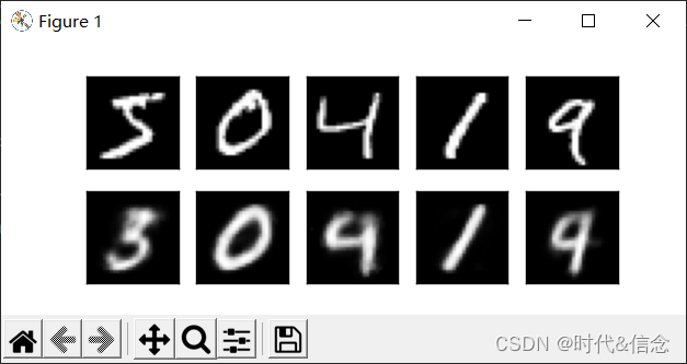
# original data (first row) for viewing
view_data = train_data.train_data[:N_TEST_IMG].view(-1, 28*28).type(torch.FloatTensor)/255.
for i in range(N_TEST_IMG):
a[0][i].imshow(np.reshape(view_data.data.numpy()[i], (28, 28)), cmap='gray'); a[0][i].set_xticks(()); a[0][i].set_yticks(())
# 训练
for epoch in range(EPOCH):
for step, (x, b_label) in enumerate(train_loader):
b_x = x.view(-1, 28*28) # batch x, shape (batch, 28*28)
b_y = x.view(-1, 28*28) # batch y, shape (batch, 28*28)
encoded, decoded = autoencoder(b_x)
# 比对解码出来的数据和原始数据,计算loss
loss = loss_func(decoded, b_y) # mean square error
optimizer.zero_grad() # clear gradients for this training step
loss.backward() # backpropagation, compute gradients
optimizer.step() # apply gradients
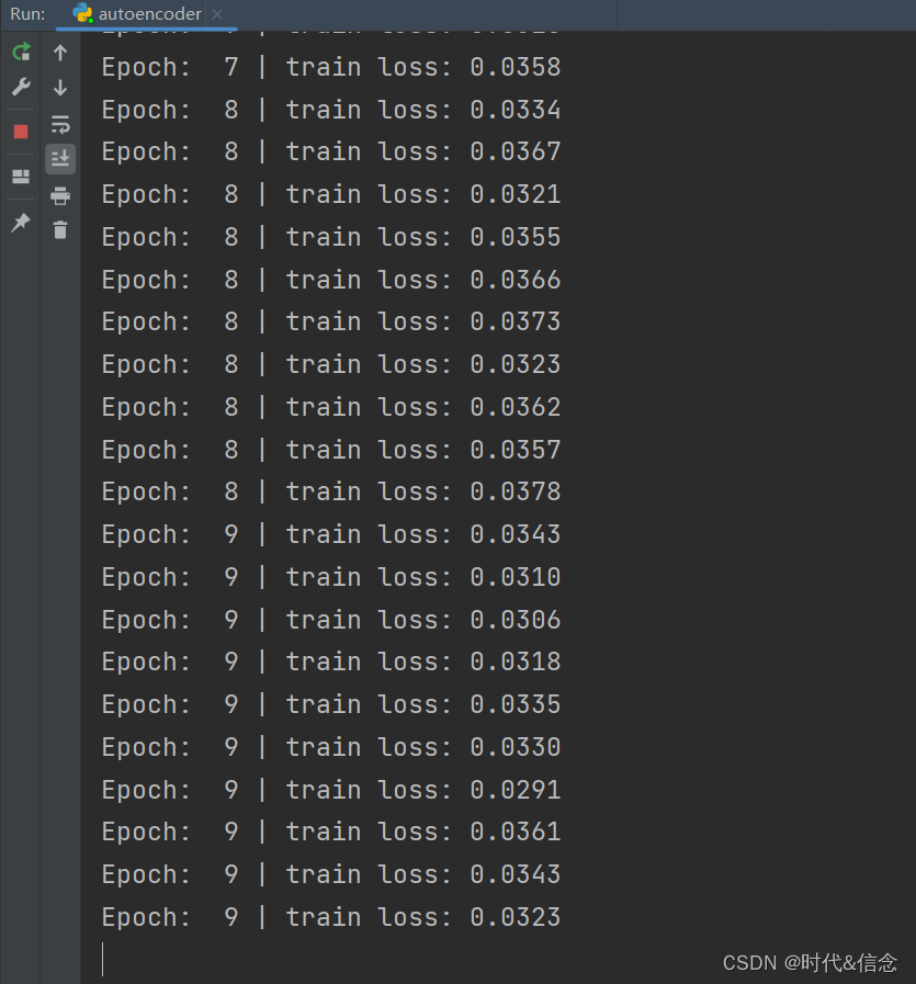
if step % 100 == 0:
print('Epoch: ', epoch, '| train loss: %.4f' % loss.data.numpy())
# plotting decoded image (second row)
_, decoded_data = autoencoder(view_data)
for i in range(N_TEST_IMG):
a[1][i].clear()
a[1][i].imshow(np.reshape(decoded_data.data.numpy()[i], (28, 28)), cmap='gray')
a[1][i].set_xticks(())
a[1][i].set_yticks(())
plt.draw()
plt.pause(0.05)
plt.ioff()
plt.show()
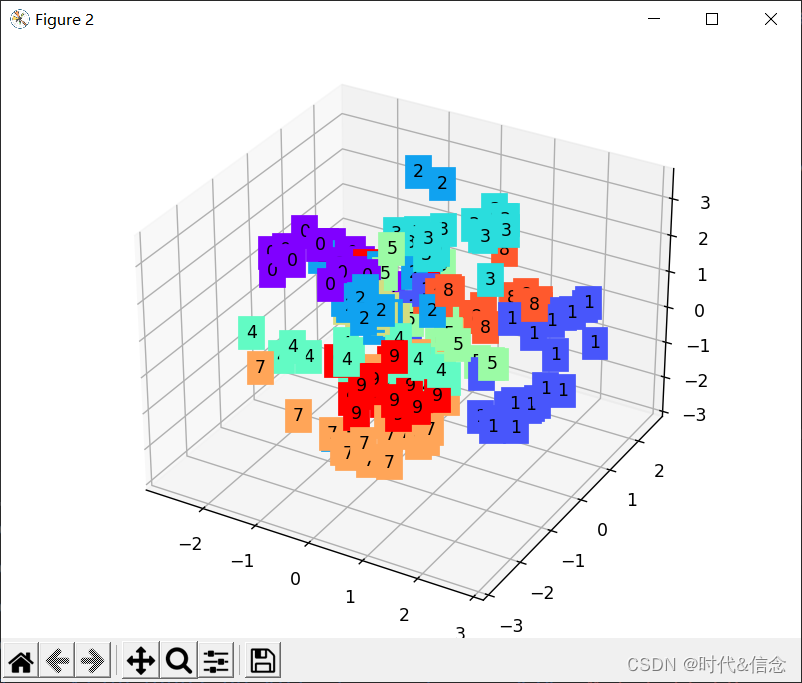
# visualize in 3D plot
view_data = train_data.train_data[:200].view(-1, 28*28).type(torch.FloatTensor)/255.
encoded_data, _ = autoencoder(view_data)
fig = plt.figure(2)
ax = Axes3D(fig)
X, Y, Z = encoded_data.data[:, 0].numpy(), encoded_data.data[:, 1].numpy(), encoded_data.data[:, 2].numpy()
values = train_data.train_labels[:200].numpy()
for x, y, z, s in zip(X, Y, Z, values):
c = cm.rainbow(int(255*s/9)); ax.text(x, y, z, s, backgroundcolor=c)
ax.set_xlim(X.min(), X.max()); ax.set_ylim(Y.min(), Y.max()); ax.set_zlim(Z.min(), Z.max())
plt.show()
operation result