TensorFlow from the encoder (AutoEncoder) Practice of MNIST

 

The effect of the encoder can be used for dimension reduction, add noise study can be obtained from the de-noising.

The following single hidden layer using the training data set mnist and shared weights symmetrical weight parameters.

The model itself is not difficult, the debugging process there are several places to note:

• The initial value of a weight parameter model sensitive to the right, so here do some limitations on the weighting parameter w
• The need for data standardization
• Learning rate set reasonable (Adam, 0.001)

1, model

Import numpy AS NP
 Import tensorflow TF AS 

class AutoEncoder (Object):
     '' ' 
    using the weight parameters of a symmetrical structure, the decoder reuse encoder 
    ' '' 
    DEF  the __init__ (Self, input_shape, h1_size, LR): 
        tf.reset_default_graph () # FIG reset the default calculation, sometimes after an error memory further mess 
        with tf.variable_scope ( ' auto_encoder ' , Reuse = tf.AUTO_REUSE): 
            self.W1 = self.weights (Shape = (input_shape, h1_size), = name ' h1 of ' ) 
            self.b1 = self.bias (h1_size) 
            self.W2 = tf.transpose (tf.get_variable ('h1'))  # 共享参数，使用其转置
            self.b2 = self.bias(input_shape)
        self.lr = lr
        self.input = tf.placeholder(shape=(None, input_shape),
                                    dtype=tf.float32)
        self.h1_out = tf.nn.softplus(tf.matmul(self.input, self.W1) + self.b1)# softplus，类relu
        self.out = tf.matmul(self.h1_out, self.W2) + self.b2
        self.optimizer = tf.train.AdamOptimizer(learning_rate=self.lr)
        self.loss = 0.1 * tf.reduce_sum(
            tf.pow(tf.subtract(self.input, self.out), 2))
        self.train_op = self.optimizer.minimize(self.loss)
        self.sess = tf.Session()
        self.sess.run(tf.global_variables_initializer())

    def fit(self, X, epoches=100, batch_size=128, epoches_to_display=10):
        batchs_per_epoch = X.shape[0] // batch_size
        for i in range(epoches):
            epoch_loss = []
            for j in range(batchs_per_epoch):
                X_train X-= [J * the batch_size: (J +. 1) * the batch_size] 
                Loss, _ = self.sess.run ([self.loss, self.train_op], 
                                        feed_dict = {self.input: X_train}) 
                epoch_loss.append (Loss ) 
            IF I% epoches_to_display == 0:
                 Print ( ' avg_loss AT Epoch% D: F% ' % (I, np.mean (epoch_loss)))
 #          return self.sess.run (W1 of) 


#      weight initialization reference others, this is actually very important! With their own set of normally distributed random truncation has no effect 
    DEF weights (Self, Shape, name, Constant =. 1 ): 
        fan_in = Shape [0]
        fan_out = shape[1]
        low = -constant * np.sqrt(6.0 / (fan_in + fan_out))
        high = constant * np.sqrt(6.0 / (fan_in + fan_out))
        init = tf.random_uniform_initializer(minval=low, maxval=high)
        return tf.get_variable(name=name,
                               shape=shape,
                               initializer=init,
                               dtype=tf.float32)

    def bias(self, size):
        return tf.Variable(tf.constant(0, dtype=tf.float32, shape=[size]))

    def encode(self, X):
        return self.sess.run(self.h1_out, feed_dict={self.input: X})

    def decode(self, h):
        return self.sess.run(self.out, feed_dict={self.h1_out: h})

    def reconstruct(self, X):
        return self.sess.run(self.out, feed_dict={self.input: X})

2, the data loading and pretreatment

from keras.datasets Import MNIST 
(X_train, y_train), (X_test, android.permission.FACTOR.) = mnist.load_data () 

Import Random 
X_train = X_train.reshape (-1, 784 )
 # test set 10 in a random test image used 
test_idxs = random .sample (Range (X_test.shape [0]), 10 ) 
data_test = X_test [test_idxs] .reshape (-1, 784 )
 # normalized 
Import sklearn.preprocessing AS Prep 
Processer = prep.StandardScaler (). Fit (X_train) # here is good with all the data, this is also very critical! 
= X_train processer.transform (X_train) 
X_test =processer.transform (data_test) 

# random 5000 pictures used as training 
idxs = random.sample (the Range (X_train.shape [0]), 5000 ) 
data_train = X_train [idxs]

3, training

= AutoEncoder Model (784, 200, 0.001)   # learning rate is a bit big impact on the loss 
model.fit (data_train, batch_size = 128, Epoches = 200)   # 200 Lun can

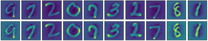
4, testing, visual comparison of FIG.

decoded_test = model.reconstruct(X_test)

import matplotlib.pyplot as plt
%matplotlib inline
shape = (28, 28)
fig, axes = plt.subplots(2,10,
                         figsize=(10, 2),
                         subplot_kw={
                             'xticks': [],
                             'yticks': []
                         },
                         gridspec_kw=dict(hspace=0.1, wspace=0.1))
for i in range(10):
    axes[0][i].imshow(np.reshape(X_test[i], shape))
    axes[1][i].imshow(np.reshape(decoded_test[i], shape))
plt.show()

The results are as follows:

 

 Above, you can add Gaussian noise at the input point, increasing robustness.