Mathematical Foundations of Artificial Intelligence--Probability and Statistics 15: Multidimensional Random Variables/Vectors

1. Definition of multidimensional random variable

Generally, let X=(X1,X2,···,X,) be an n-dimensional vector , and each of its components, that is, X1,···,Xn is a one-dimensional random variable, then X is said to be an n dimensional random vector or n-dimensional random variable .

Like random variables, random vectors can also be divided into discrete and continuous types.

2. Discrete multidimensional random vector

A random vector X=(X1,···,Xn), if each component Xi is a one-dimensional discrete random variable, then X is called discrete.

2.1. Probability of discrete multidimensional random vectors

Definition 2.1
$$with{a}_i,a_{i2},\cdot \cdot \cdot remember{X}_{i}All\; possible\; values\; ofi(=1,2,\cdot \cdot \cdot ),\; then\; eventX1=a_{1j_1},X2\_=a_{2j_2},\cdot \cdot \cdot ,Xn=a_{n{j}_n}The\; probability\; of\; is\; called\; a\; random\; vector,$$
recorded as:

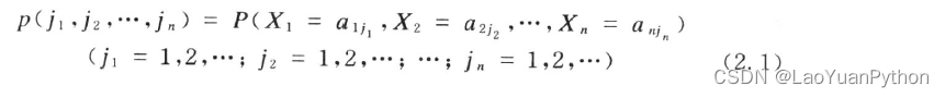
X=(X1,···,Xn) probability function or probability distribution, the probability function should meet the conditions:

2.2, multinomial distribution

Multinomial distribution is the most important discrete multidimensional distribution, which is often encountered in practice. For example, when a population is divided into several categories according to attributes, it is multinomial distribution.

2.2.1 Definition

Let A1, A2, ..., An be a complete event group under a certain experiment, that is, events A1, ..., An are mutually exclusive, and their sum is an inevitable event (events A1, · ··, An must occur one and only one). Take P1, P2, ···, Pn to record the probability of events A1, A2, ···, An respectively, then pi≥0, P1+···+pn=1.
Now the experiment is repeated N times independently, and Xi records the number of occurrences of event Ai in these N experiments (i=1,...,n), then X=(X1,...,Xn) is an n dimensional random vector. Its value range is: X1, ..., Xn are all non-negative integers, and their sum is N. The probability distribution of X is called a multinomial distribution , sometimes denoted as M(N; P1,...,Pn) .

2.2.2 Calculation method

In order to determine this distribution, to calculate the probability of event B=(X1=k1,···,Xi=Ki,···,Xn=Kn}, just consider that Ki is a non-negative integer and K1+···+Kn =N, otherwise P(B)=0.

To calculate P(B), start from the raw results j1,j2,···,jN of N trials, which represent the occurrence of the first trial event Aj1, the second trial Aj2 occurrence, and so on. For event B to occur, there should be k1 of 1s, k2 of 2s in j1, j2, . . . , jN, and so on. The number of such sequences is equal to dividing N different objects into n piles, and each pile has k1, k2, ..., kn pieces of different divisions in turn. There are N!/(k1!···kn!) kinds of divisions. Secondly, due to independence, using the probability multiplication theorem, the probability of occurrence of each original result sequence j1j2···jn that meets the above conditions should be $p_1^k{p}_2^{k2}\cdot \cdot \cdot p_n^{kn}$. Then we get:

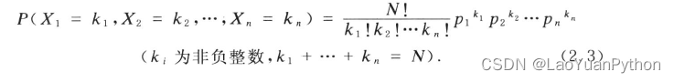
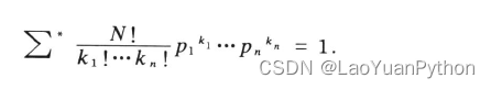
the above formula is the probability function of multinomial distribution, and its name is multinomial expansion:

$S^{\ast }indicates\; that\; the\; range\; of\; summation\; is:k_{i}is\; a\; non-negative\; integer,k1+\cdot \cdot \cdot +kn=N.$ _
In the above formula, let xi=pi, and use p1+···+pn=1, get:

3. Continuous multidimensional random variable

3.1 Definition

Suppose X=(X1,···,Xn) is an n-dimensional random vector, and its value can be regarded as an n-dimensional Euclidean space $R^{}$A point in${}^n$$R^{A\; region\; in\; n}$ is called a continuousmultidimensional random variable.

Like a one-dimensional continuous variable, the most convenient way to describe the probability distribution of a multidimensional random vector is to use a probability density function. To this end, we introduce a notation: X∈A, read "X belongs to A" or "X falls within A", where A is $R^{The\; set\; in\; n}$ : {XE∈A} is a random event, because after doing the experiment, the value of X is known, so it can also be known whether it falls in A.

3.2 Probability Density Functions of Multidimensional Random Variables

Definition If f(x1,···,xn) is defined in $R^{}$non-negative function on${}^n$$R^{}$For any set A in${}^n$

, there is: Then f is said to be the (probability) density function of X.
If A is taken as the full space$R^n$ , then {X∈A} is an inevitable event with a probability of 1. So there should be

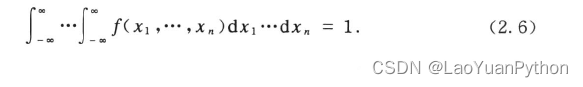
This is also a condition that the probability density function must satisfy.

3.3 Uniform distribution

Two-dimensional random vector X=(X1,X2), its probability density function is:

Then f is non-negative and satisfies formula (2.6).

The graph corresponding to this function is as follows:

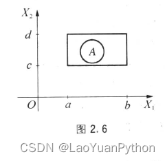
All probabilities are evenly distributed in the corresponding rectangle, that is, P(X∈A) is proportional to the area of ​​A, so the distribution of X is called the uniform distribution on the rectangle in the figure .

3.6 Two-dimensional normal distribution

The most important multidimensional continuous distribution is the multidimensional normal distribution. The probability density function of the two-dimensional normal distribution

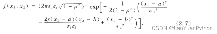
in the two-dimensional case is as follows: Here, for convenience, the symbol exp is introduced, and its meaning is: exp(c) = $e^c$ . The above probability density function contains 5 constants a, b,$p_1^2、p_2^2$, ρ, they are the parameters of the two-dimensional normal distribution, and their possible value ranges are:
a, b∈(-∞, +∞), $p_1>0、p_2>0$，ρ∈（-1,1）

Two-dimensional normal distribution is often recorded as N(a, b, $p_1^2、p_2^2$, ρ) , its function graph in three-dimensional space is like an ellipse-sectioned bell upside down on the Ox1x2 plane, and its center is at point (a, b).

can prove N(a，b，$p_1^2、p_2^2$, **ρ)** satisfies the requirements of formula (2.6), so this is a probability density function.

3.7 Points to note about continuous random variables

1. Whether it is a one-dimensional or multi-dimensional continuous random variable, the essence of the definition is that there needs to be a probability density function (for one-dimensional is a variable) that satisfies the formula (2.6);
2. Whether the probability density function is continuous in an interval or area is not required;
3. Each component of a continuous random vector is a random variable, but it is not necessarily a random vector if each component is a random variable;
4. The probability distribution function can be used to describe the probability distribution of multidimensional random vectors, which is defined as: F(x1,x2,…,xn)=P(X1<x1,X2<x2,…,Xn<xn), but in the case of multidimensional Next, the distribution function is rarely used.

3.8 Marginal distribution

Let X=(X1,...,Xn) be an n-dimensional random vector, X has a certain distribution F, which is an n-dimensional distribution, because each component Xi of X is a one-dimensional random variable, so they have their own The distribution Fi(i=1,···,n), these are one-dimensional distribution, called the marginal distribution of the random vector X or its distribution F , also known as the marginal distribution . The marginal distribution is completely determined by the original distribution F.

3.8.1 Marginal distribution of discrete random vectors

Taking the first component as an example, the formula for calculating the probability density of the marginal distribution of discrete random vectors is:

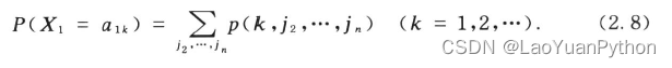
It can be proved that for the multinomial distribution M(N;p1,...,pn), the corresponding marginal distribution is the binomial distribution B (N,pi).

3.8.2 Marginal distribution of continuous random vectors

Suppose the random vector X=(X1,...,Xn) has a probability density function f(x1,...,xn), the probability density function of the marginal distribution of its component Xi is to fix xi, and the remaining n-1 variables of the function f Do a definite integral between -∞ and +∞, such as under the density function of x1:

In this way, it can be proved that the marginal distribution of the two-dimensional normal distribution is a one-dimensional normal distribution.

Four. Summary

This paper introduces the concept of multidimensional random vectors, the definition of their probability density function and the definition of marginal distribution, and gives examples of typical distributions of multidimensional random vectors such as multinomial distribution, uniform distribution, and normal distribution. Multidimensional random vectors are also divided into two types: discrete and continuous. The marginal distribution is a common distribution, but one or more components are regarded as variables, and the rest of the components are distributions obtained by global integration. Therefore, the marginal distribution can be It can be one-dimensional or multi-dimensional.
Corresponding to the marginal distribution, the multidimensional random vector is also called the joint distribution .

The distribution F of any random vector can determine the marginal distribution Fi of one of its components, but even knowing the marginal distribution Fi of all components is not enough to determine the distribution F of the random vector . For example, if the parameter ρ of two standard normal distributions is different, the two are respectively regarded as the marginal distribution of the two-dimensional random vector, and the corresponding random vectors are different distributions. This is because the marginal distribution only considers the case of a single component and does not consider its relationship.

For more artificial intelligence mathematical foundations, please refer to the column " [Artificial Intelligence Mathematical Foundations] One-Dimensional (https://blog.csdn.net/laoyuanpython/category_10382948.html)".

Blogging is not easy, please support:

If you have gained something from reading this article, please like, comment, and bookmark, thank you for your support!

Paid Columns About Old Ape

1. The paid column " https://blog.csdn.net/laoyuanpython/category_9607725.html Using PyQt to Develop Graphical Interface Python Applications" specifically introduces the basic tutorial of Python-based PyQt graphical interface development, and the corresponding article directory is " https://blog.csdn .net/LaoYuanPython/article/details/107580932 Use PyQt to develop a graphical interface Python application column directory ";
2. The paid column " https://blog.csdn.net/laoyuanpython/category_10232926.html moviepy audio and video development column ) introduces in detail the class-related methods of moviepy audio and video clip synthesis processing and the use of related methods to process related clip synthesis scenes, corresponding articles The directory is " https://blog.csdn.net/LaoYuanPython/article/details/107574583 moviepy audio and video development column article directory ";
3. The paid column " https://blog.csdn.net/laoyuanpython/category_10581071.html OpenCV-Python Beginners Difficult Questions Collection " is " https://blog.csdn.net/laoyuanpython/category_9979286.html OpenCV-Python Graphics and Image Processing "The accompanying column is the integration of the author's personal perception of some problems encountered in the learning of OpenCV-Python graphics and image processing. To understand OpenCV, the corresponding article directory is " https://blog.csdn.net/LaoYuanPython/article/details/109713407 OpenCV-Python Beginners Difficult Problem Collection Column Directory "
4. The paid column " https://blog.csdn.net/laoyuanpython/category_10762553.html Getting Started with Python Crawlers" introduces what you should know about crawler development from the perspective of an Internet front-end development novice, including the basics of getting started with crawlers, and how to crawl. Get CSDN article information, blogger information, give articles likes, comments and other actual combat content.

The first two columns are suitable for novice readers who have a certain Python foundation but no relevant knowledge. The third column please combine " https://blog.csdn.net/laoyuanpython/category_9979286.html OpenCV-Python Graphics and Image Processing " learning to use.

For colleagues who lack the foundation of Python, you can learn Python from scratch through Lao Yuan's free column " https://blog.csdn.net/laoyuanpython/category_9831699.html Column: Python Basic Tutorial Catalog ).

If you are interested and willing to support Laoyuan readers, you are welcome to purchase paid columns.

Old Ape Python, learn Python from Old Ape!

☞ ░ Go to Laoyuan Python blog post directory https://blog.csdn.net/LaoYuanPython ░