
1. The definition of the probability density function of a continuous random variable
- In " Mathematical Foundations of Artificial Intelligence – Probability and Statistics 10: Probability Functions of Discrete Random Variables and Common Binomial Distribution and Poisson Distribution ", the concept of probability distribution function is introduced: Let X be a random variable (including discrete and non-discrete), Then the function: P(X≤x) = F(x) (-∞ < x <∞) is called the distribution function of X ;
- Suppose a continuous random variable X has a probability distribution function F(x), then the derivative f(x)=F'(x) of F(x) is called the probability density function of X, or density function for short .
2. Properties of the probability density function of a continuous random variable
The density function f(x) of a continuous random variable X has the following three basic properties:
- f(x)≥0;
- ∫ − ∞ + ∞ f ( x ) d ( x ) = 1 \int^{+∞}_{-∞}f(x)d(x) = 1 ∫−∞+∞f(x)d(x)=1
- For any constant a less than b, we have: P ( a ≤ X ≤ b ) = F ( b ) − F ( a ) = ∫ abf ( x ) d ( x ) P(a≤X≤b)=F(b) -F(a)=\int^b_af(x)d(x)P(a≤X≤b)=F(b)−F(a)=∫abf(x)d(x)
3. Normal distribution
3.1. Definition
If a random variable has the following probability density function:
f ( x ) = ( 2 π σ ) − 1 e − ( x − u ) 2 2 σ 2 ( − ∞ < x < ∞ ) {\Large f(x) = ( \sqrt{2π} \;σ )^{-1}e^{-\frac{(xu)^2}{2σ^2}}} \;\;\;\;\;\;\;\; \;\;(-∞<x<∞)f(x)=(2 p.ms )− 1 e−2 p2(x−u)2(−∞<x<∞ )
, then X is calleda normal random variable, and it is recorded as: X ~ N(u,σ²), where u and σ² are constants, u is any real number, 0<σ<∞ (the original writing is σ², the old Ape thinks that σ should be greater than 0), u and σ² are the "parameters" of the normal distribution.
3.2. Proof that the normal distribution is a probability density function
To prove that the normal distribution f(x) is a probability density function is to prove that:
- f(x)≥0, since σ is greater than 0, f(x) is obviously greater than or equal to 0;
- ∫ − ∞ ∞ f ( x ) dx = 1 , 即 ∫ − ∞ ∞ ( 2 π σ ) − 1 e − ( x − u ) 2 2 σ 2 dx = 1 ∫^∞_{-∞}f(x) dx=1,即∫^∞_{-∞} (\sqrt{2π} \;σ )^{-1}e^{-\frac{(xu)^2}{2σ^2}}dx=1∫−∞∞f(x)dx=1 , that is∫−∞∞(2 p.ms )− 1 e−2 p2(x−u)2dx=1
to perform variable substitution, set t=(xu)/σ, then it is necessary to prove:∫ − ∞ ∞ e − t 2 2 dt = 2 π ∫^∞_{-∞} e^{-\frac{t^2 }{2}}dt= \sqrt{2π}∫−∞∞e−2t2dt=2 p.m
\\
Old Ape Note : First of all, explain why it is necessary to prove that ∫ − ∞ ∞ e − t 2 2 dt = 2 π ∫^∞_{-∞} e^{-\frac{t^2}{2}}dt= \sqrt {2π}∫−∞∞e−2t2dt=2 p.m
∵ ∫ ( 2 π σ ) − 1 e − ( x − u ) 2 2 σ 2 dx ∴ ( 2 π ) − 1 ∫ e − ( x − u ) 2 2 σ 2 dx σ ∴ ( 2 π ) − 1 ∫ e − t 2 2 d ( t − u σ ) ∴ 即要 证明 : I = ∫ − ∞ ∞ e − t 2 2 dt = 2 π ∵∫(\sqrt{2π} \;σ )^{-1} e^{-\frac{(xu)^2}{2σ^2}} dx\\∴(\sqrt{2π} )^{-1}∫e^{-\frac{(xu)^2}{ 2σ^2}} d\frac{x}{σ}\\∴(\sqrt{2π} )^{-1}∫e^{-\frac{t^2}{2}} d(t-\ frac{u}{σ})\\∴即要要要:I = ∫^∞_{-∞} e^{-\frac{t^2}{2}}dt= \sqrt{2π}∵∫(2 p.ms )− 1 e−2 p2(x−u)2dx∴(2 p.m)−1∫e−2 p2(x−u)2dpx∴(2 p.m)−1∫e−2t2d(t−pu)∴That is to prove that : I=∫−∞∞e−2t2dt=2 p.m
Next, carry out the proof of this formula:
Since the integral variable does not affect the integral result, we can get: I ² = ∫ − ∞ ∞ e − t 2 2 dt ∫ − ∞ ∞ e − u 2 2 du = ∫ − ∞ ∞ ∫ − ∞ ∞ e − t 2 + u 2 2 dtdu \\I²= ∫^∞_{-∞} e^{-\frac{t^2}{2}}dt ∫^∞_{-∞} e^{-\ frac{u^2}{2}}du= ∫^∞_{-∞} ∫^∞_{-∞} e^{-\frac{t^2+u^2}{2}} dt duI²=∫−∞∞e−2t2dt∫−∞∞e−2u2of u=∫−∞∞∫−∞∞e−2t2+u2Convert d t d u
into polar coordinates, let t=rcosθ, u=rsinθ, then:
I ² = ∫ 0 2 π d θ ∫ 0 ∞ e − r ² / 2 rdr = 2 π × ∫ 0 ∞ e − r ² / 2 dr ² 2 I²= ∫^{2π}_0 dθ ∫^∞_0e^{-r²/2}rdr = 2π× ∫^∞_0e^{-r²/2}d\frac{r²}{2}I²=∫02 p.md i∫0∞e−r²/2rdr=2 p.m×∫0∞e−r²/2d2r²
Let y = r²/2, then the range of definite integral is still [0, ∞), then:
I ² = 2 π × ∫ 0 ∞ e − ydy = − 2 π × ∫ 0 ∞ e − yd ( − y ) = − 2 π × e − y ∣ 0 ∞ = 2 π I²= 2π× ∫^∞_0e^{-y}dy=-2π× ∫^∞_0e^{-y}d(-y)=-2π×e^{ -y}|^∞_0=2πI²=2 p.m×∫0∞e− the dy=− 2 p×∫0∞e− y d(−y)=− 2 p×e−y∣0∞=2 π
So we can get:I = 2 π I=\sqrt{2π}I=2 p.m, the proof is completed.
3.3. The graph of normal distribution and its application examples
The function graph of the normal distribution is as follows:
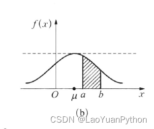
From the above image, it can be seen that the function is symmetrical about point u, the middle is high and the two ends are low. This state is the state of general things, such as a person's height, weight, income, size A certain index of the same product manufactured in batches conforms to the normal distribution to varying degrees, which not only explains the origin of the normal (Normal) distribution, but also illustrates the importance of this distribution.
Four. Summary
This article introduces the concepts of probability distribution and probability density function of continuous random variables, and introduces an important probability density function of continuous random variables: the definition, derivation and usage scenarios of the probability density function of normal distribution.
For more mathematical foundations of artificial intelligence, please refer to the column " Mathematical Foundations of Artificial Intelligence ".
Blogging is not easy, please support:
If you have gained something from reading this article, please like, comment, and bookmark, thank you for your support!
Paid Columns About Old Ape
- The paid column " https://blog.csdn.net/laoyuanpython/category_9607725.html Using PyQt to Develop Graphical Interface Python Applications" specifically introduces the basic tutorial of Python-based PyQt graphical interface development, and the corresponding article directory is " https://blog.csdn .net/LaoYuanPython/article/details/107580932 Use PyQt to develop a graphical interface Python application column directory ";
- The paid column " https://blog.csdn.net/laoyuanpython/category_10232926.html moviepy audio and video development column ) introduces in detail the class-related methods of moviepy audio and video clip synthesis processing and the use of related methods to process related clip synthesis scenes, corresponding articles The directory is " https://blog.csdn.net/LaoYuanPython/article/details/107574583 moviepy audio and video development column article directory ";
- The paid column " https://blog.csdn.net/laoyuanpython/category_10581071.html OpenCV-Python Beginners Difficult Questions Collection " is " https://blog.csdn.net/laoyuanpython/category_9979286.html OpenCV-Python Graphics and Image Processing "The accompanying column is the integration of the author's personal perception of some problems encountered in the learning of OpenCV-Python graphics and image processing. To understand OpenCV, the corresponding article directory is " https://blog.csdn.net/LaoYuanPython/article/details/109713407 OpenCV-Python Beginners Difficult Problem Collection Column Directory "
- The paid column " https://blog.csdn.net/laoyuanpython/category_10762553.html Getting Started with Python Crawlers" introduces what you should know about crawler development from the perspective of an Internet front-end development novice, including the basics of getting started with crawlers, and how to crawl. Get CSDN article information, blogger information, give articles likes, comments and other actual combat content.
The first two columns are suitable for novice readers who have a certain Python foundation but no relevant knowledge. The third column please combine " https://blog.csdn.net/laoyuanpython/category_9979286.html OpenCV-Python Graphics and Image Processing " learning to use.
For colleagues who lack the foundation of Python, you can learn Python from scratch through Lao Yuan's free column " https://blog.csdn.net/laoyuanpython/category_9831699.html Column: Python Basic Tutorial Catalog ).
If you are interested and willing to support Laoyuan readers, you are welcome to purchase paid columns.