[PubMed Mathematics] Probability Theory and Mathematical Statistics——Chapter Two | One-dimensional random variables and their distributions (1, basic concepts and common types of random variables)

---

introduction

The summer vacation is coming to an end, so try to catch up with the progress of the probability theory part.

---

1. One-dimensional random variable and its distribution

1.1 Random variables

EE $The\; sample\; space\; of\; E$ is$Oh$，$X$ is defined in the sample spaceΩ \OmegaA function on$\Omega$$w\in \Omega$ , there is always a uniquely determined$X\left(w\right)$ corresponds to it, called$X\left(w\right)$ is a random variable, generally denoted as$X$ 。

A certain value range of a random variable is essentially a random event. If the random variable cannot take any value within a certain range, it is essentially an impossible event. If a certain range includes all possible values ​​​​of the random variable, it is essentially a random event. inevitable event.

1.2 Distribution function

Let $X$ is a random variable, for any real number$x$ , said function$F(x)=P$ { $X\le x$ } is a random variableXXThe distribution function of$X.$

It has the following four properties:

（1）$0\le F\left(x\right)\le 1;$

（2）$F\left(x\right)$ isxxa monotonically nondecreasing function of$x\; ;$

（3）$F\left(x\right)$ about$x$ right continuous;

（4）$F(-\infty )=0,F(+\infty )=1.$

If there is a function that satisfies the above four conditions, it can be called the distribution function of a random variable. Such as $F(3x-1)$ is still a distribution function, but$F(1-3x)$ is not a distribution function, when$x\to +\infty$ ，$F(1-3x)$ the limit is 0 but not 1;$F(x^2)$is not a distribution function either, because when$x\to +\infty$ ，$F\left(x^2\right)$The limit is 1 but not 0.

Let random variable $The\; distribution\; function\; of\; X$ is$F\left(x\right)$ , then
(1)$P$ { $X<a$ } $=F(a-0);$
（2）$P$ { $a<X\le b$ } $=F(b)-F(a);$
（3）$P$ { $a\le X<b$ } $=F(b-0)-F(a-0);$
（4）$P$ { $a\le X\le b$ } $=F(b)-F(a-0);$
（5）$P$ { $a<X<b$ } $=F(b-0)-F(a);$
（6）$P$ { $X=a$ } $=F(a)-F(a-0);$

---

2. Common types and distributions of random variables

2.1 Discrete random variable

Let $X$ is a random variable, if$The\; possible\; values\; of\; X$ are finite or listable, called$X$ is a discrete random variable.

Let the discrete random variable XXThe possible values ​​of$X$$x_i(i=1,2,\dots )$ , the corresponding probability is$P$ { $X=x_i$ } $=p_i$, called $P$ { $X=x_i$ } $=p_i$or the table below

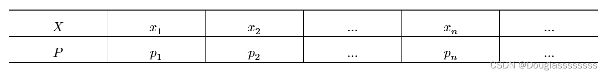
is the random variable XXThe distribution law of$X.$

Discrete random variable $The\; distribution\; law\; of\; X$ satisfies:
(1)$p_i\ge 0(i=1,2,\dots ).$
（2）${\sum }_{i=1}^{+\infty }{p}_i=1.$
(3) Distribution function$F(x)=P$ { $X\le x$ } is a step function, and$The\; discontinuity\; point\; of\; F\left(x\right)$ is the random variableXXPossible values ​​of$X.$

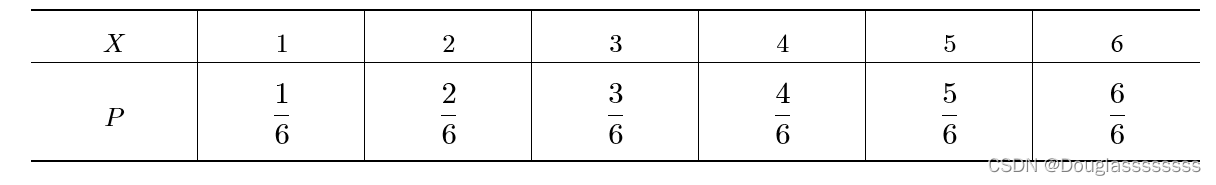
What is a step function, that is, the image is like a step. For example, remember the random variable $X$ is the point of throwing an even dice, then$X$ can be$1,2,3,4,5,6$ , and$P$ { $X=i$ } $=\frac{1}{6}(i=1,2,\dots ,6)$ , its distribution law is shown in the following table:

The image of the distribution function is:

Note that the ladder is right first and then up. Because it is a discrete value, the value of the distribution function between two values ​​should be the function value corresponding to the previous value.

2.2 Continuous random variable and probability density function

Let random variable $The\; distribution\; function\; of\; X$ is$F\left(x\right)$ , if there exists a non-negative, integrable function$f\left(x\right)$ , such that for any real number$x$ ，有 $$F(x)={\int }_{-\infty }^{x}f\left(t\right)dt,$$ called$X$ is a continuous random variable, the function$f\left(x\right)$ is a random variableXXThe probability density function or probability density of$X.$

The probability density of continuous random variables has the following conclusions:

（1）$f(x)\ge 0;$

（2）${\int }_{-\infty }^{+\infty }f(t)dt=1;$

(3) Distribution function $F\left(x\right)$ is a continuous function, but not necessarily derivable;

（4）$P$ { $X=a$ } $=F(a)-F(a-0)=0$ , so the probability of a continuous random variable at any point is 0 .

(5) Let the distribution function be $F\left(x\right)$ , then the probability density function is$$f(x)=\{\begin{array}{ll}{F}^{\prime }(x),& x\text{is}a\; derivable\; point\; ofF\left(x\right)\\ 0,& xisa\; non-differentiable\end{array}$$(6) There are random variables that are neither discrete nor continuous, such as random variable XXThe distribution function expression of$X$$$F(x)=\{\begin{array}{ll}0,& \text{if }x<0\\ \frac{x}{2},& \text{if }0\le x<1\\ 1& \text{if }x\ge 1\end{array}$$Obviously $F\left(x\right)$ satisfies the four characteristics of the distribution function, but it is not a step function, so$X$ is a non-discrete random variable. And becauseF ( x ) F(x)There are discontinuities in$F$$($$x$$)$$X$ is also a non-continuous random variable, and its image is shown in the figure below.

---

write at the end

In the next article we will introduce some common random variable distributions.