YOLO works on a single-stage detection principle, which means it unifies all components of the object detection pipeline into a single neural network. It uses features from the entire image to predict class probabilities and bounding box coordinates.
This approach facilitates global reasoning modeling of the entire image and objects within the image. However, in previous two-stage detectors like RCNN, we have a proposal generator that generates rough proposals for images, which are then passed to the next stage for classification and regression.

Recommendation: Use NSDT Designer to quickly build programmable 3D scenes.
1. Overview of YOLO model
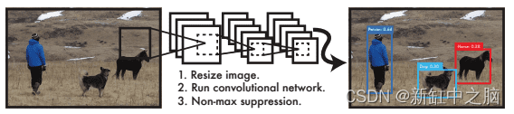
The figure below shows that the entire detection process consists of three steps: resizing the input image to 448 × 448, running a single convolutional network on the full image, and thresholding the resulting detections based on the confidence of the model, thereby eliminating duplicate detections.
This end-to-end unified detection design enables the YOLO architecture to train faster and achieve real-time speed during inference, while ensuring high average accuracy (close to two-stage detectors).
Traditional approaches such as DPM use a sliding window approach. However, the classifier operates on uniformly distributed locations across the image, so training and testing times are very slow, and optimization is challenging, especially for RCNN architectures since each stage needs to be trained individually.
We understand that YOLO works on a unified end-to-end detection approach, but how does it achieve this goal? Let's find out!
The YOLO model divides the image into an S × S grid, as shown in Fig. 5, where S = 7. This unit is responsible for detecting an object if its center falls into one of the 49 grids.
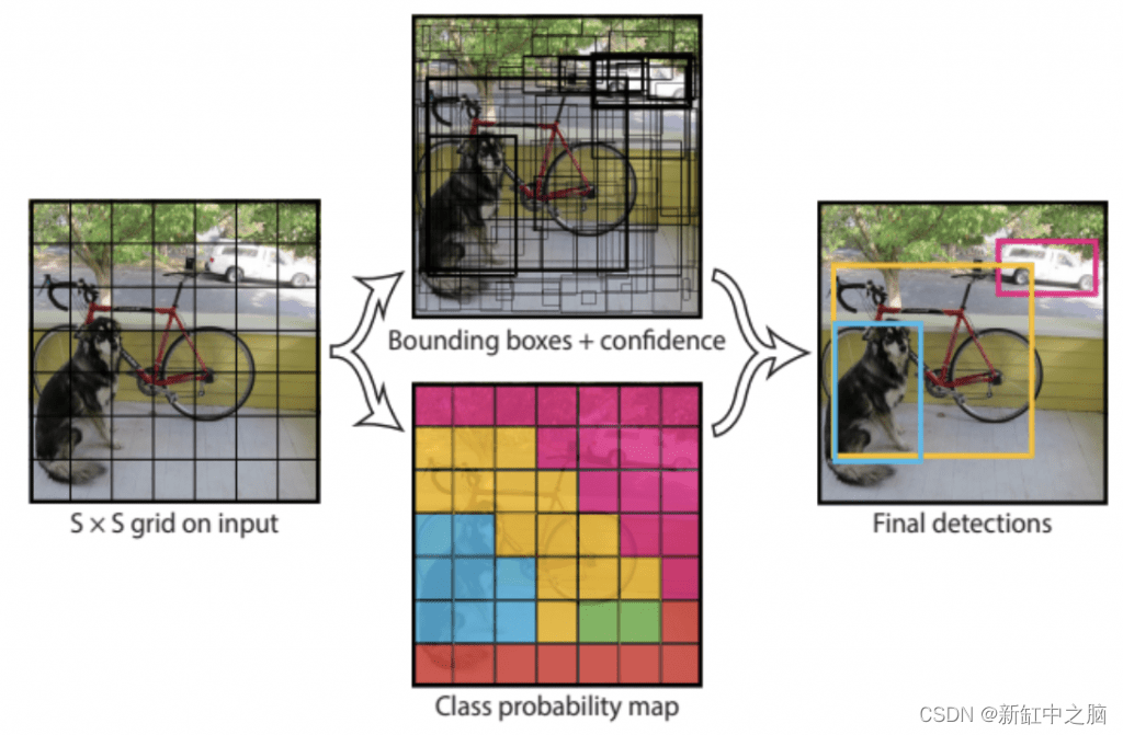
But how many objects can a grid cell be responsible for detecting? Then, each grid cell can detect B bounding boxes and the confidence scores of these bounding boxes, B = 2.
In total, the model can detect 49 × 2 = 98 bounding boxes; however, as we will see later, during training, the model tries to suppress one of the two boxes in each cell that has fewer intersection unions (IOUs) with the ground truth box.
Each box is assigned a confidence score that indicates how confident the model is that the bounding box contains the object.
The confidence score can be defined as:
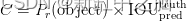
where Pr(object) is 1 if the object exists, and 0 otherwise; when an object exists, the confidence score is equal to the IOU between the ground truth and the predicted bounding box.
This makes sense because we don't want a confidence score of 100% (1) when the predicted box is not perfectly aligned with the ground truth, which allows our network to predict a more realistic confidence for each bounding box.
Outputs five predictions per bounding box:
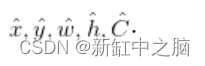
- The target (x, y) coordinates represent the center of the bounding box relative to the grid cell boundary, which means that (x, y) has values in the range [0, 1]. An (x, y) value of (0.5, 0.5) indicates that the center of the object is the center of a particular grid cell.
- Target(w,h) is the width and height of the bounding box relative to the entire image. This means that the predicted (w_hat, h_hat) will also be relative to the whole image. The width and height of the bounding box can be greater than 1.
- C_hat is the confidence score predicted by the network.
In addition to bounding box coordinates and confidence scores, each grid cell predicts C conditional class probabilities Pr(Classi|Object), where C = 20 for PASCAL VOC classes. Pr is conditional on the grid cell containing the object; therefore, it only exists if there is an object.
We learned that each grid cell is responsible for predicting two boxes. However, only the one with the highest IOU to the ground truth is considered; thus, the model predicts a set of class probabilities for each grid cell, ignoring the number of boxes B.
To develop more intuition, see the figure below; we can observe a 7 × 7 grid, each grid cell has output predictions for Box 1 and Box 2 and class probabilities.
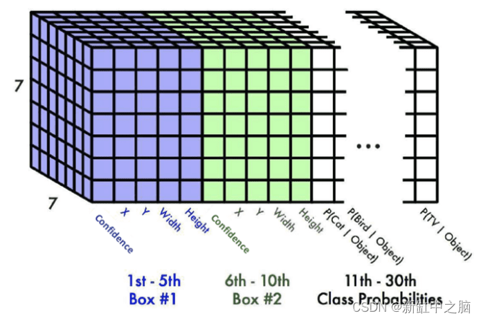
Each bounding box has five values [confidence, X, Y, Width, Height], for a total of 10 values for the bounding box and 20 class probabilities. Therefore, the final prediction is a 7 × 7 × 30 tensor.
2. YOLO's network architecture
YOLO's network architecture is very simple, trust me! It's similar to image classification networks you've trained in the past. But, surprisingly, the architecture was inspired by the GoogLeNet model used in image classification tasks.
It mainly consists of three types of layers: convolutional layers, max pooling layers, and fully connected layers. The YOLO network has 24 convolutional layers to extract image features, followed by two fully connected layers to predict bounding box coordinates and classification scores.
Modified the original GoogLenet architecture by Redmond et al. First, they use 1 × 1 convolutional layers instead of inception modules to reduce the feature space, followed by 3 × 3 convolutional layers:
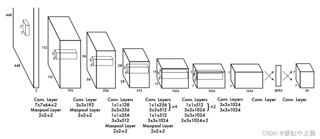
The second variant of YOLO, called Fast-YOLO, has 9 convolutional layers (instead of 24) and uses smaller filter sizes. The main purpose is to further increase the speed of reasoning to a level that people cannot imagine. With this setup, the author was able to achieve 155 FPS!
3. YOLO's loss function design
Let us now dissect the YOLO loss function shown in Figure 9. At first glance, the equation below might look a bit lengthy and tricky, but don't worry; it's easy to understand.
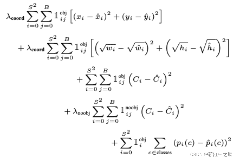
You'll notice that in this loss equation, we're optimizing the network using sum squared error (SSE) and Redmon et al. I believe it is easy to optimize. However, there are some caveats to using it, which they try to overcome by adding a weight term called lambda.
Let's break down the equation above:
- The first part of the equation computes the loss between the predicted bounding box midpoint (x_hat, y_jat) and the true bounding box midpoint (x, y).
It is computed for all 49 grid cells and only one of the two bounding boxes is considered in the loss. Remember that it only penalizes the bounding box coordinate error of the predictor that is "responsible" for the ground truth box (ie, the predictor with the highest IOU in that grid cell).
In short, we will see the two bounding boxes that have the highest IOU with the target bounding box, and will be prioritized for loss calculation.
Finally, we scale the loss with a constant lambda_coord=5 to ensure our bounding box predictions are as close to the target as possible. Finally, 1^obj_ij means that the jth bounding box predictor in cell i is responsible for the prediction. So it's 1 if the target object exists, 0 otherwise.
- The second part is very similar to the first, so let's go over the differences. Here we compute the loss between the predicted bounding box width and height (w_hat, h_hat) and the target width and height (w, h).
Note, however, that we take the square root of width and height (i.e., because the sum-of-squares loss weighs error in both large and small boxes equally).
Significant deviations in small boxes will be small, while small changes in large boxes will be significant, causing small boxes to decrease in importance. Therefore, the authors added a square root to reflect that slight deviations in large boxes have less effect than in small boxes.
- In the third part of the equation, given the existence of an object 1^\obj_ij=1, we compute the loss between the bounding box's predicted confidence score C_hat and the target confidence score {C}.
Here, the object confidence score C is equal to the IOU between the predicted bounding box and the object. We select the confidence score of the box with higher IOU from the target.
- Next, 1^noobj_ij=1 and 1^obj_ij=0 will make the third part of the equation zero if no object exists in grid cell i. The loss is computed between the box with the higher IOU and the target C, which is 0, because we want the confidence to be 0 for cells without objects.
We also scale this with lambda_noobj=0.5, since there may be many grid cells without objects, and we don't want this term to overwhelm the gradient of cells containing objects. As highlighted in this paper, this can make the model unstable and more difficult to optimize.
Finally, for each cell, 1^obj_i=1 if an object occurs in cell i, we compute the loss (conditional class probabilities) for all 20 classes. Here, p_hat© is the predicted conditional class probability and p© is the target conditional class probability.
Original link: Intuition of YOLO model — BimAnt