The technology behind the open source large model BLOOM with hundreds of billions of parameters

Suppose you now have the data and the budget, everything is ready, and you are ready to start training a large model. Once you show off your skills, "seeing all the flowers in Chang'an in one day" seems to be just around the corner... Wait a minute! Training is not as simple as the pronunciation of these two words. It may be helpful to see BLOOM's training.

In recent years, it has become the norm for language models to get bigger and bigger. People usually criticize that the information of these large models themselves is not disclosed for research, but little attention is paid to the knowledge behind the large model training technology. This article aims to take the language model BLOOM with 176 billion parameters as an example to clarify the software and hardware engineering and technical points behind training such models, so as to promote the discussion of large model training technology.

First, we would like to thank the companies, individuals, and groups that enabled or sponsored our group's culmination of the incredible feat of training a 176 billion parameter model.

Then, we start discussing the hardware configuration and main technical components.

The following is a brief summary of the project:

hardware	384 80GB A100 GPUs
software	Megatron-DeepSpeed
model architecture	Based on GPT3
data set	350 billion words in 59 languages
training time	3.5 months

Staff composition

The project was conceived by Thomas Wolf (Co-Founder and CSO of Hugging Face), who dared to compete with the big companies, proposing not only to train a model that stands on the world's largest forest of multilingual models, but also to make it available to everyone Public access to training results fulfills most people's dreams.

This article focuses on the engineering aspects of model training. Some of the most important parts of the technology behind BLOOM are the people and companies who share their expertise and help us code and train.

We mainly need to thank 6 groups:

1. HuggingFace's BigScience team devoted more than six full-time employees to the research and operation of the training, and they also provided or reimbursed for all infrastructure other than Jean Zay's computer.
2. The developers of the Microsoft DeepSpeed ​​team, which developed DeepSpeed ​​and later integrated it with Megatron-LM, spent weeks researching the project's requirements and provided a lot of great practical advice before and during training.
3. The NVIDIA Megatron-LM team that developed Megatron-LM have been more than happy to answer our many questions and provide top-notch usage advice.
4. The IDRIS/GENCI team, which manages the Jean Zay supercomputer, donated significant computing power and strong system administration support to the project.
5. The PyTorch team has created a powerful framework on which the rest of the software is based and has been very supportive in preparing us for training, fixing several bugs and improving the training usability of the PyTorch components we depend on.
6. BigScience Engineering Working Group Volunteer

It's hard to name all the brilliant people who contributed to the engineering side of the project, so I'll just name a few key people outside of Hugging Face who laid the engineering groundwork for the project over the past 14 months:

Olatunji Ruwase、Deepak Narayanan、Jeff Rasley、Jared Casper、Samyam Rajbhandari 和 Rémi Lacroix

We also thank all companies that allowed their employees to contribute to this project.

overview

The model architecture of BLOOM is very similar to GPT3 with some improvements, which are discussed later in this paper.

The model was trained on Jean Zay, a French government-funded supercomputer managed by GENCI and installed at IDRIS, the national computing center of the French National Center for Scientific Research (CNRS). The computing power required for training is generously donated to this project by GENCI (donation number 2021-A0101012475).

Training hardware:

• GPU: 384 NVIDIA A100 80GB GPUs (48 nodes) + 32 spare GPUs
• 8 GPUs per node, 4 NVLink inter-card interconnects, 4 OmniPath links
• CPU: AMD EPYC 7543 32-core processor
• CPU memory: 512GB per node
• GPU memory: 640GB per node
• Inter-node connection: Omni-Path Architecture (OPA) network card is used, and the network topology is a non-blocking fat tree
• NCCL - Communications Network: a fully dedicated subnetwork
• Disk IO network: GPFS shared with other nodes and users

Checkpoints:

• main checkpoints
• Each checkpoint contains an optimizer state with a precision of fp32 and a weight with a precision of bf16+fp32, and occupies a storage space of 2.3TB. If only the weight of bf16 is saved, only 329GB of storage space will be occupied.

data set:

• 1.5TB of heavily deduplicated and cleaned text in 46 languages, converted to 350B tokens
• The model's vocabulary contains 250,680 tokens
• For more details, please refer to The BigScience Corpus A 1.6TB Composite Multilingual Dataset

The training of the 176B BLOOM model took about 3.5 months to complete from March to July 2022 (about 1 million computing hours).

Megatron-DeepSpeed

The 176B BLOOM model is trained using Megatron-DeepSpeed , which combines two main techniques:

• Megatron-DeepSpeed:
• DeepSpeed ​​is a deep learning optimization library that makes distributed training simple, efficient and effective.
• Megatron-LM is a large and powerful transformer model framework developed by NVIDIA's applied deep learning research team.

The DeepSpeed ​​team developed a 3D parallel-based scheme by combining ZeRO sharding and Pipeline Parallelism in the DeepSpeed ​​library with Tensor Parallelism in Megatron-LM. See the table below for more details on each component.

Please note that BigScience's Megatron-DeepSpeed ​​is based on the original Megatron-DeepSpeed ​​code base, and we have added quite a few codes to it.

The following table lists which components of each of the two frameworks we employ when training BLOOM:

components	DeepSpeed	Megatron-LM
ZeRO Data Parallel	yes
Tensor Parallel		yes
Pipeline Parallel	yes
BF16 optimizer	yes
CUDA fusion kernel function		yes
data loader		yes

Note that both Megatron-LM and DeepSpeed ​​have pipelined parallelism and BF16 optimizer implementations, but we use DeepSpeed's implementation because they are integrated into ZeRO.

Megatron-DeepSpeed ​​achieves 3D parallelism to allow large models to be trained in a very efficient manner. Let's briefly discuss what 3D components are.

1. Data Parallelism (DP) - The same setup and model are replicated multiple times, each fed with a different copy of the data each time. Processing is done in parallel, with all shares synchronized at the end of each training step.
2. Tensor Parallelism (TP) - Each tensor is split into chunks, so each slice of the tensor resides on its assigned GPU, rather than having the entire tensor reside on a single GPU. During processing, each shard is processed separately and in parallel on a different GPU, and the results are synchronized at the end of the step. This is called horizontal parallelism, because it is done horizontally.
3. Pipeline Parallelism (PP) - The model is split vertically (ie, by layer) across multiple GPUs so that only one or more model layers are placed on a single GPU. Each GPU processes different stages of the pipeline in parallel and processes a portion of the batch.
4. Zero Redundancy Optimizer (ZeRO) - also performs tensor sharding similar to TP, but the entire tensor is rebuilt in time for forward or reverse computation, so no model modifications are required. It also supports various offloading techniques to compensate for limited GPU memory.

data parallelism

Most users with only a few GPUs are probably familiar with DistributedDataParallel(DDP), which is the corresponding PyTorch documentation . In this approach, the models are fully replicated to each GPU, and then all models synchronize their states with each other after each iteration. This method can speed up training and solve problems by investing more GPU resources. But it has the limitation that it only works if the model fits on a single GPU.

ZeRO Data Parallel

The following diagram nicely depicts ZeRO data parallelism (from this blog post ).

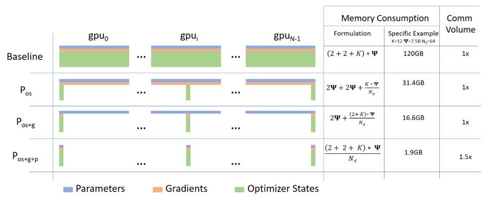
It seems to be relatively tall, which may make it difficult for you to concentrate on understanding, but in fact, the concept is very simple. This is just the usual DDP, except that instead of each GPU replicating the full model parameters, gradients, and optimizer state, each GPU only stores a portion of it. During subsequent runs, when the full layer parameters for a given layer are required, all GPUs synchronize to provide each other with their missing pieces - nothing more.

This component is implemented by DeepSpeed.

Tensor Parallel

In Tensor Parallelism (TP), each GPU processes only a portion of a tensor, and aggregation operations are triggered only when certain operators require the full tensor.

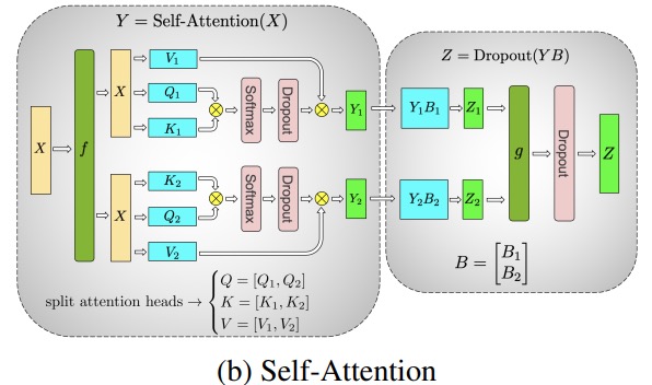
In this section we use concepts and diagrams from the Megatron-LM paper Efficient Large-Scale Language Model Training on GPU Clusters .

The main modules of the Transformer class model are: a fully connected layer nn.Linearfollowed by a non-linear activation layer GeLU.

Following the notation from the Megatron paper, we can write the dot product part as Y = GeLU (XA), where Xand Yare the input and output vectors, Aand is the weight matrix.

It's easy to see how matrix multiplication can be split across multiple GPUs if expressed in matrix form:

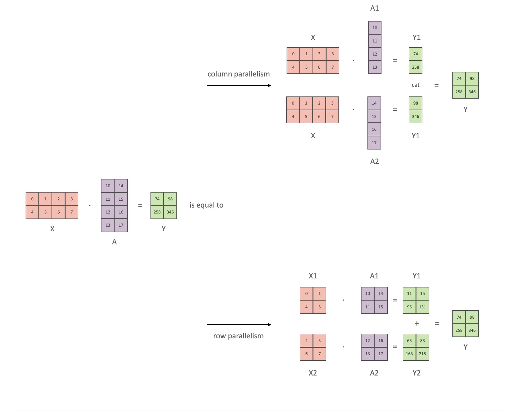
If we split the weight matrices Aby columns Nonto GPUs, and then perform matrix multiplications XA_1in XA_n, then we end up Nwith output vectors Y_1、Y_2、…… 、 Y_n, which can be fed independently GeLU:

Note that because Ythe matrix is ​​split by column, we can choose the row-wise splitting scheme for the subsequent GEMM, so that it can directly get the output of the GeLU of the previous layer without any additional communication.

Using this principle, we can update an MLP of arbitrary depth, simply by synchronizing the GPU after each 拆列 - 拆行sequence . The authors of the Megatron-LM paper provide a nice illustration for this:

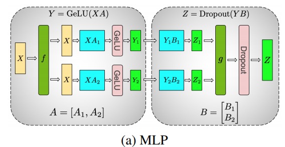
Here fis the identity operator in the forward pass and all reduce in the backward pass, and gis the all reduce in the forward pass and the identity in the backward pass.

Parallelizing multi-head attention layers is even simpler since they are inherently parallel due to multiple independent heads!

Special considerations: Since there are two all-reduces per layer in the forward and backward passes, TP requires very fast interconnects between devices. Therefore, unless you have a very fast network, it is not recommended to do TP across multiple nodes. In our hardware configuration for training BLOOM, the speed between nodes is much slower than PCIe. In fact, if the node has 4 GPUs, a maximum TP degree of 4 is better. If you need a TP degree of 8, you need to use a node with at least 8 GPUs.

This component is implemented by Megatron-LM. Megatron-LM has recently expanded the tensor parallel capability, and added the capability of sequence parallelism for operators that are difficult to use the aforementioned segmentation algorithm, such as LayerNorm. The Reducing Activation Recomputation in Large Transformer Models paper provides details of this technique. Sequence parallelism was developed after training BLOOM, so BLOOM was trained without this technique.

Pipeline Parallel

Naive pipeline parallelism (naive PP) is to distribute model layers in groups across multiple GPUs and simply move data from GPU to GPU as if it were one large composite GPU. The mechanism is relatively simple - you bind the desired layer to the corresponding device with .to()the method , and now whenever data enters or exits these layers, the layers will switch the data to the same device as the layer, and the rest remains the same.

This is actually vertical model parallelism, because if you remember how we draw the topology of most models, we actually split the layers of the model vertically. For example, if the image below shows an 8-layer model:

=================== ===================
| 0 | 1 | 2 | 3  | |  4 | 5 | 6 | 7 |
=================== ===================
        GPU0 GPU1

We cut it vertically into 2 parts, placing layers 0-3 on GPU0 and layers 4-7 on GPU1.

Now, when data is passed from layer 0 to layer 1, layer 1 to layer 2, and layer 2 to layer 3, it's just like normal forward pass on a single GPU. But when data needs to pass from layer 3 to layer 4, it needs to be transferred from GPU0 to GPU1, which introduces communication overhead. If the participating GPUs are on the same compute node (eg, the same physical machine), the transfer is very fast, but if the GPUs are on different compute nodes (eg, multiple machines), the communication overhead can be much larger.

Then layers 4 to 5 to 6 to 7 are like normal models again, and when layer 7 is done we usually need to send data back to layer 0 where the labels are (or send the labels to the last layer). Now the loss can be calculated and the optimizer can be used to update the parameters.

question:

• Why is this method called naive pipeline parallelism, and what are its drawbacks? Mainly because the scheme has all but one GPU idle at any given moment. So if you use 4 GPUs, you're almost quadrupling the amount of memory on a single GPU, and other resources (like compute) are pretty much useless. Add in the overhead of copying data between devices. So 4 6GB cards in parallel using naive pipeline will be able to hold the same size model as 1 24GB card which trains faster because it has no data transfer overhead. But, for example, if you have a 40GB card, but need to run a 45GB model, you can use 4x 40GB cards (which is just enough, because there are also gradients and optimizer states that require video memory).
• Sharing embeddings may require copying back and forth between GPUs. The pipelined parallelism (PP) we use is almost the same as the naive PP above, but it solves the GPU idling problem by chunking incoming batches into micros batches and artificially creating pipelines that allow different GPUs to participate in the computation process simultaneously.

The figure below is from the GPipe paper , the upper part represents the naive PP scheme, and the lower part is the PP method:

From the bottom half of the figure it is easy to see that PP has less dead zone (meaning the GPU is idle), ie less "bubbles".

The degree of parallelism of the two schemes in the figure is 4, that is, the pipeline is composed of 4 GPUs. So there are four forward paths of F0, F1, F2, and F3, and then the reverse path of B3, B2, B1, and B0.

PP introduces a new hyperparameter to tune, called 块 (chunks). It defines how many blocks of data are sent sequentially through the same pipe level. For example, in the bottom half of the figure, you can see chunks = 4. GPU0 executes the same forward path on chunks 0, 1, 2, and 3 (F0,0, F0,1, F0,2, F0,3) and then waits until the other GPUs finish their work before GPU0 starts working again , execute the backward path for blocks 3, 2, 1, and 0 (B0,3, B0,2, B0,1, B0,0).

Note that this is conceptually the same as gradient accumulation steps (GAS). PyTorch calls it 块, and DeepSpeed ​​calls it GAS.

Because 块, PP introduces the concept of micro-batches (MBS). DP splits the global batch size into small batch sizes, so if the DP degree is 4, the global batch size 1024 will be split into 4 small batch sizes, and each small batch size is 256 (1024/4). And if 块the number (or GAS) is 32, we end up with a micro batch size of 8 (256/32). Each tube stage processes one micro batch at a time.

The formula to calculate the global batch size for the DP+PP setting is: mbs * chunks * dp_degree( 8 * 32 * 4 = 1024).

Let's go back and look at the picture again.

Using naive PP chunks=1you end up with naive PP, which is very inefficient. And with very large 块numbers , you end up with small micro-batch sizes, which are probably not very efficient either. Therefore, one must experiment to find 块the number .

The graph shows that there are "dead" time bubbles that cannot be parallelized because the last forwardstage has to wait for backwardthe pipeline to finish. Then, the problem of finding the optimal 块number so that all participating GPUs can achieve high concurrent utilization is actually transformed into minimizing the number of bubbles.

This scheduling mechanism is called 全前全后. Some other options are Tandem and Interleaved Tandem .

While both Megatron-LM and DeepSpeed ​​have their own implementations of the PP protocol, Megatron-DeepSpeed ​​uses the DeepSpeed ​​implementation because it is integrated with other features of DeepSpeed.

Another important issue here is the size of the word embedding matrix. While generally word embedding matrices require less memory than transformer blocks, in the case of BLOOM with a 250k vocabulary, the embedding layer requires 7.2GB for bf16 weights, compared to only 4.9GB for the transformer block. Therefore, we had to make Megatron-Deepspeed treat the embedding layer as a transformer block. So we have a pipeline of 72 stages, 2 of which are dedicated to embedding (first and last). This allows us to balance the memory consumption of the GPU. If we didn't do this, we would have the first and last stages consume a lot of GPU memory, and 95% of the GPU memory usage would be very little, so the training would be very inefficient.

DP+PP

There is a picture in the DeepSpeed ​​Pipeline Parallel Tutorial that demonstrates how to combine DP and PP, as shown below.

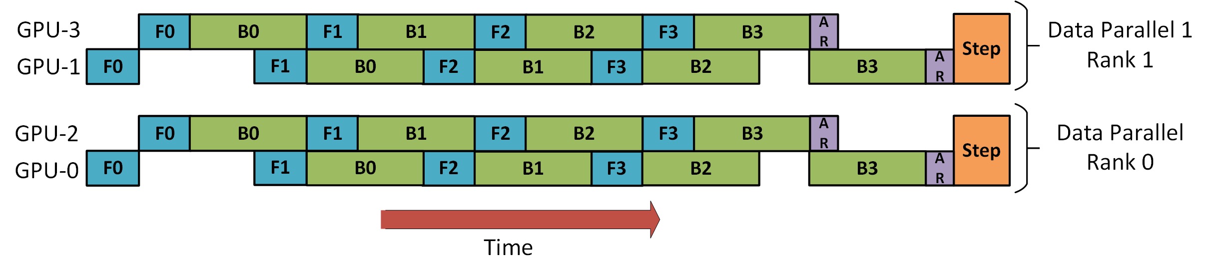
The important thing to understand here is that DP rank 0 cannot see GPU2, and DP rank 1 cannot see GPU3. For DP, there are only GPUs 0 and 1, and data is fed to them. GPU0 uses PP to "secretly" offload some of its load to GPU2. Likewise, GPU1 will also get help from GPU3.

Since at least 2 GPUs are required for each dimension, at least 4 GPUs are required here.

DP+PP+TP

For more efficient training, PP, TP, and DP can be combined, called 3D parallelism, as shown in the figure below.

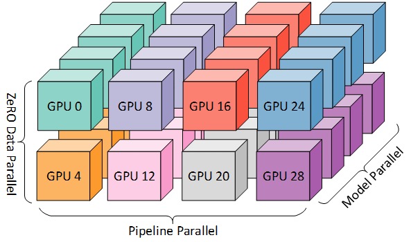
This figure is from the blog post 3D Parallelism: Scaling to Trillion Parameter Models ), which is also a good article.

Since you need at least 2 GPUs per dimension, here you need at least 8 GPUs for full 3D parallelism.

ZeRO DP+PP+TP

One of the main features of DeepSpeed ​​is ZeRO, which is a super-scalable enhanced version of DP, which we have discussed in the section [ZeRO Data Parallel] (#ZeRO- Data Parallel). Usually it is an independent function and does not require PP or TP. But it can also be combined with PP, TP.

When ZeRO-DP is combined with PP (and thus TP), it typically only enables ZeRO phase 1, which only shards the optimizer state. ZeRO stage 2 also shards gradients, and stage 3 also shards model weights.

While it is theoretically possible to use ZeRO stage 2 with pipeline parallelism, it can have a bad impact on performance. Each micro batch requires an additional reduce-scatter communication to aggregate gradients before sharding, which adds potentially significant communication overhead. According to the parallel nature of the pipeline, we will use small micro batches, and focus on the trade-off between arithmetic intensity (micro batch size) and minimizing pipeline bubbles (number of micro batches). Therefore, the increased communication overhead hurts pipeline parallelism.

Also, due to PP, the number of layers is already less than normal, so it doesn't save much memory. PP has reduced the gradient size 1/PP, so the gradient slice on this basis does not save much memory compared to pure DP.

ZeRO stage 3 can also be used to train models of this size, however, it requires more communication than DeepSpeed ​​3D in parallel. A year ago, after careful evaluation of our environment, we found that Megatron-DeepSpeed ​​3D parallelism performed best. The performance of ZeRO Phase 3 has improved significantly since then, and if we were to re-evaluate it today, maybe we would choose Phase 3.

BF16 optimizer

Training huge LLM models with FP16 is a no-no.

We've demonstrated this for ourselves by spending months training the 104B model, which, as you can see from Tensorboard , failed utterly. In the process of fighting against the ever-diverging lm-loss, we learned a lot:

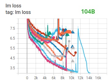
We also got the same suggestion from the Megatron-LM and DeepSpeed ​​teams after they trained the 530B model . The recently released OPT-175B also reported that they trained very hard on FP16.

So back in January we knew we were going to train on the A100 which supports the BF16 format. Olatunji Ruwase developed a "BF16Optimizer" for training BLOOM.

If you are not familiar with this data format, check out its bit layout . The key to the BF16 format is that it has the same number of exponents as FP32, so it won't overflow, but FP16 often overflows! FP16 has a maximum value range of 64k, you can only multiply smaller numbers. For example you can do 250*250=62500, but if you try 255*255=65025, you will overflow, which is the main cause of problems with training. This means your weights must be kept small. A technique called loss scaling helps alleviate this problem, but FP16's small range can still be an issue when models get very large.

The BF16 doesn't have this problem, you can do it easily 10_000*10_000=100_000_000, no problem at all.

Of course, since BF16 and FP16 are the same size, 2 bytes, there is no free lunch, and the tradeoff when using BF16 is that it has very poor precision. However, you should remember that the stochastic gradient descent method and its variants we used in training, this method is a bit like staggering, if you don't find the perfect direction at this step, it's okay, you will correct it in the next step Own.

Whether using BF16 or FP16, there is a copy of the weights that is always in FP32 - this is what is updated by the optimizer. So the 16-bit format is only used for calculations, the optimizer updates the FP32 weights with full precision, and then converts them to 16-bit format for the next iteration.

All PyTorch components have been updated to ensure that they perform any accumulation in FP32, so no loss of precision occurs.

A key issue is gradient accumulation, which is one of the main features of pipeline parallelism, since the gradients processed by each micro-batch are accumulated. Implementing gradient accumulation in FP32 for training accuracy is critical, and this is exactly BF16Optimizerwhat was done .

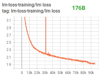
Among other improvements, we believe that using BF16 mixed-precision training turned a potential nightmare into a relatively smooth process, as can be seen in the following lm loss plot:

CUDA fusion kernel function

The GPU mainly does two things. It can write data to and read data from video memory and perform computations on that data. When the GPU is busy reading and writing data, the computing units of the GPU are idle. If we want to utilize the GPU efficiently, we want to keep idle time to a minimum.

A kernel function is a set of instructions that implement a specific PyTorch operation. For example, torch.addwhen , it goes through a PyTorch scheduler , which decides which code it should run based on the values ​​of the input tensors and other variables, and finally runs it. CUDA kernels use CUDA to implement these codes and therefore only run on NVIDIA GPUs.

Now, c = torch.add (a, b); e = torch.max ([c,d])when , typically what PyTorch will do is launch two separate kernels, one that does the addition aof band , cand the other that takes the maximum of dboth . In this case, the GPU afetches bthe sum from its video memory, performs the addition, and then writes the result back to video memory. It then takes cand dand performs maxthe operation , and writes the result back to video memory again.

If we were to fuse these two operations, i.e. put them into a "fused kernel function", and then launch that kernel, instead of cwriting it in GPU registers, and only need Gets dto do the final calculation. This saves a lot of overhead and prevents the GPU from idling, so the whole operation is much more efficient.

The fusion kernel function does just that. They primarily replace multiple discrete computations and data movement to and from video memory with fused computations with very little data movement. Additionally, some fusion kernels mathematically transform operations so that certain combinations of calculations can be performed faster.

In order to train BLOOM quickly and efficiently, it is necessary to use several custom CUDA fused kernel functions provided by Megatron-LM. In particular, there is a LayerNorm fusion kernel and kernels for various combinations of fusion scaling, masking, and softmax operations. Bias Add is also integrated with GeLU through PyTorch's JIT function. These operations are all memory-bound, so it is important to fuse them together to maximize the amount of computation after each video memory read. So, for example, executing Bias Add while executing a GeLU operation whose bottleneck is in memory will not increase the running time. These kernel functions can be found in the Megatron-LM code library .

data set

Another important feature of Megatron-LM is the efficient data loader. Before the first training starts, each sample in each dataset is divided into samples of fixed sequence length (BLOOM is 2048), and an index is created to number each sample. Based on the training hyperparameters, we will determine the number of epochs that each dataset needs to participate in, and based on this, create an ordered list of sample indices, and then shuffle it. For example, if a dataset has 10 samples that should be trained for 2 epochs, the system first sorts the sample indices in [0, ..., 9, 0, ..., 9]order then shuffles the order to create the final global order for the dataset. Note that this means that the training will not simply iterate over the entire dataset and repeat, you may see the same sample twice before seeing another, but at the end of training the model will only see each sample twice Second-rate. This helps ensure a smooth training curve throughout training. These indices, including the offset of each sample in the original dataset, are saved to a file to avoid recomputing them each time training is started. Finally, several of these datasets can be blended with different weights into the final data used for training.

Embed LayerNorm

In our efforts to prevent the divergence of the 104B model, we found that adding an additional LayerNorm after the first word embedding layer made the training more stable.

This insight comes from experiments with bitsandbytes , which has an operation which is a normal embedding with a LayerNorm initialized with a uniform xavier function.StableEmbedding

location code

Based on the paper Train Short, Test Long: Attention with Linear Biases Enables Input Length Extrapolation , we also replace the normal positional embeddings with AliBi, which allows extrapolation of input sequences longer than the input sequences used to train the model. Therefore, even though we train with sequences of length 2048, the model can handle longer sequences during inference.

difficulties in training

With the architecture, hardware and software in place, we were able to start training in early March 2022. Since then, however, things have not been all smooth sailing. In this section, we discuss some of the main obstacles we encountered.

Before training begins, there are a lot of questions to figure out. In particular, we found several issues that only appeared after we started training on 48 nodes, not at small scales. For example, CUDA_LAUNCH_BLOCKING=1to prevent the framework from hanging, we need to divide the optimizer group into smaller groups, otherwise the framework will hang again. You can read more about these in the Pre-Training Chronicles.

The main type of problems encountered during training are hardware failures. Since this is a new cluster with about 400 GPUs, on average we experience 1-2 GPU failures per week. We save a checkpoint every 3 hours (100 iterations). As a result, we lose an average of 1.5 hours of training per week to hardware crashes. Jean Zay system administrator will then replace the faulty GPU and restore the node. In the meantime, we have spare nodes available.

We've also had various other issues that resulted in 5-10 hour downtime multiple times, some related to deadlock bugs in PyTorch, others due to insufficient disk space. If you're interested in specifics, see the training chronicle .

All of this downtime was planned for in the feasibility analysis of training this model, and we chose the appropriate model size and the amount of data we wanted the model to consume accordingly. So, even with these downtime issues, we managed to complete the training within the estimated time. As mentioned earlier, it takes about 1 million compute hours to complete.

Another problem is that SLURM was not designed to be used by a group of people. SLURM jobs are owned by a single user, and if they are not around, other members of the group cannot do anything with the running job. We have a termination scheme that allows other users in the group to terminate the current process without the presence of the user who started the process. This works great on 90% of the problems. If the SLURM designers read this, please add the concept of a Unix group so that a SLURM job can be owned by a group.

Since the training runs 24/7, we need someone on call - but since we have people in Europe and the west coast of Canada, there's no need for someone to carry a pager and we're pretty good at backing each other up. Of course, weekend training has to be watched. We automate most things, including automatically recovering from hardware crashes, but sometimes human intervention is still required.

in conclusion

The most difficult and stressful part of training is the 2 months before training starts. We were under a lot of pressure to start training as soon as possible, and because of the limited time allocated by resources, we didn't get access to the A100 until the last minute. So it was a very difficult time, considering BF16Optimizerthat was written at the last minute, we needed to debug it and fix various bugs. As mentioned in the previous section, we found new problems that only appeared after we started training on 48 nodes, and not at small scales.

But once we got that sorted out, the training itself went surprisingly smoothly without major hiccups. Most of the time, there is only one of us watching, and only a few people involved in troubleshooting. We had great support from Jean Zay's management who promptly addressed most of the needs that arose during training.

Overall, it was a super intense but rewarding experience.

Training large language models remains a challenging task, but we hope that by building and sharing this technique publicly, others can learn from our experience.

resource

important link

• main training document
• Tensorboard
• slurm script for training
• training chronicle

Papers and Articles

It is impossible for us to explain everything in detail in this article, so if the techniques presented here pique your curiosity and make you want to learn more, please read the following papers:

Megatron-LM:

• Efficient Large-Scale Language Model Training on GPU Clusters.
• Reducing Activation Recomputation in Large Transformer Models

DeepSpeed:

• ZeRO: Memory Optimizations Toward Training Trillion Parameter Models
• ZeRO-Offload: Democratizing Billion-Scale Model Training
• ZeRO-Infinity: Breaking the GPU Memory Wall for Extreme Scale Deep Learning
• DeepSpeed: Extreme-scale model training for everyone

Megatron-LM and Deepspeedeed combined:

• Using DeepSpeed and Megatron to Train Megatron-Turing NLG 530B, A Large-Scale Generative Language Model.

ALiBi:

• Train Short, Test Long: Attention with Linear Biases Enables Input Length Extrapolation
• What Language Model to Train if You Have One Million GPU Hours? - There you will find the experiments that ultimately led us to choose ALiBi.

BitsNBytes:

• 8-bit Optimizers via Block-wise Quantization (we used the embedding LaynerNorm in this paper, but other parts of the paper and its techniques are also very good, the only reason we didn't use 8-bit optimizers is that we already used DeepSpeed-ZeRO to save optimizer memory).

Blog post thanks

Many thanks to the following people who asked good questions and helped improve the readability of the article (in alphabetical order):

• Britney Muller,
• Douwe Kiela,
• Jared Casper,
• Jeff Rasley,
• Julien Launay,
• Leandro von Werra,
• Omar Sanseviero,
• Stefan Schweter and
• Thomas Wang.

The charts in this article were primarily created by Chunte Lee.

---

Original English text: https://hf.co/blog/bloom-megatron-deepspeed

Original Author: Stas Bekman

Translator: Matrix Yao (Yao Weifeng), an Intel deep learning engineer, works on the application of transformer-family models on various modal data and the training and reasoning of large-scale models.

Proofreading and typesetting: zhongdongy (Adong)

{{o.name}}

{{m.name}}