Article Directory
1. Obtain data
1. Technical tools
IDE editor: vscode
Send request: requests
Analysis tool: xpath
def Get_Detail(Details_Url):
    Detail_Url = Base_Url + Details_Url
    One_Detail = requests.get(url=Detail_Url, headers=Headers)
    One_Detail_Html = One_Detail.content.decode('gbk')
    Detail_Html = etree.HTML(One_Detail_Html)
    Detail_Content = Detail_Html.xpath("//div[@id='Zoom']//text()")
    Video_Name_CN,Video_Name,Video_Address,Video_Type,Video_language,Video_Date,Video_Number,Video_Time,Video_Daoyan,Video_Yanyuan_list = None,None,None,None,None,None,None,None,None,None
    for index, info in enumerate(Detail_Content):
        if info.startswith('◎译  名'):
            Video_Name_CN = info.replace('◎译  名', '').strip()
        if info.startswith('◎片  名'):
            Video_Name = info.replace('◎片  名', '').strip()
        if info.startswith('◎产  地'):
            Video_Address = info.replace('◎产  地', '').strip()
        if info.startswith('◎类  别'):
            Video_Type = info.replace('◎类  别', '').strip()
        if info.startswith('◎语  言'):
            Video_language = info.replace('◎语  言', '').strip()
        if info.startswith('◎上映日期'):
            Video_Date = info.replace('◎上映日期', '').strip()
        if info.startswith('◎豆瓣评分'):
            Video_Number = info.replace('◎豆瓣评分', '').strip()
        if info.startswith('◎片  长'):
            Video_Time = info.replace('◎片  长', '').strip()
        if info.startswith('◎导  演'):
            Video_Daoyan = info.replace('◎导  演', '').strip()
        if info.startswith('◎主  演'):
            Video_Yanyuan_list = []
            Video_Yanyuan = info.replace('◎主  演', '').strip()
            Video_Yanyuan_list.append(Video_Yanyuan)
            for x in range(index + 1, len(Detail_Content)):
                actor = Detail_Content[x].strip()
                if actor.startswith("◎"):
                    break
                Video_Yanyuan_list.append(actor)
    print(Video_Name_CN,Video_Date,Video_Time)
    f.flush()
    try:
        csvwriter.writerow((Video_Name_CN,Video_Name,Video_Address,Video_Type,Video_language,Video_Date,Video_Number,Video_Time,Video_Daoyan,Video_Yanyuan_list))
    except:
        pass
Save data: csv
if __name__ == '__main__':
    with open('movies.csv','a',encoding='utf-8',newline='')as f:
        csvwriter = csv.writer(f)
        csvwriter.writerow(('Video_Name_CN','Video_Name','Video_Address','Video_Type','Video_language','Video_Date','Video_Number','Video_Time','Video_Daoyan','Video_Yanyuan_list'))
        spider(117)
2. Crawl target
本次爬取的目标网站是阳光电影网https://www.ygdy8.net,用到技术为requests+xpath。主要获取的目标是2016年-2023年之间的电影数据。
3. Field information
获取的字段信息有电影译名、片名、产地、类别、语言、上映时间、豆瓣评分、片长、导演、主演等,具体说明如下:
| field name | meaning |
Video_Name_CN |
film translation |
Video_Name |
movie title |
Video_Address |
film origin |
Video_Type |
movie category |
Video_language |
movie language |
Video_Date |
release time |
Video_Number |
movie rating |
Video_Time |
Length |
Video_Daoyan |
director |
Video_Yanyuan_list |
starring list |

2. Data preprocessing
Technical tool: jupyter notebook
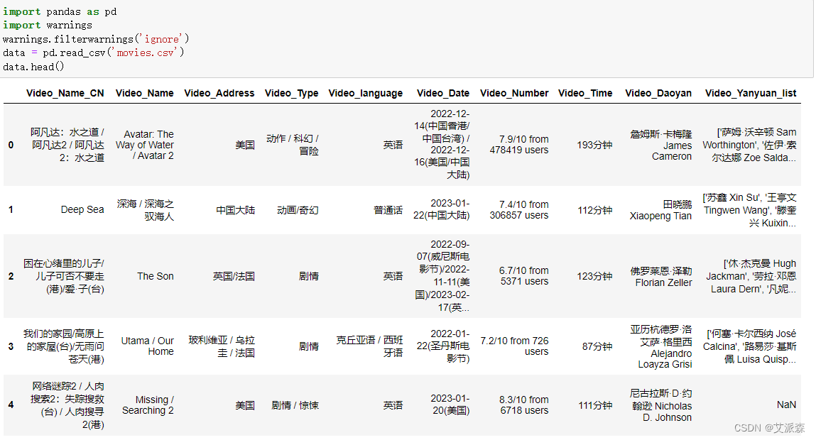
1. Load data
First use pandas to read the movie data just obtained with the crawler
2. Outlier processing
Outliers handled here include missing values and duplicate values
First check the absence of each field in the original data
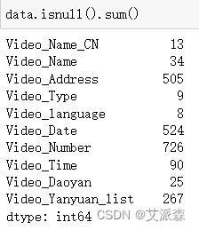
From the results, it can be found that there are quite a lot of missing data. Here, for the convenience of unified deletion processing, the duplicate data is also deleted
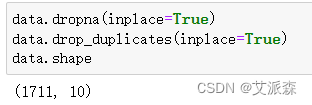
It can be found that there are 1711 pieces of processed data left.
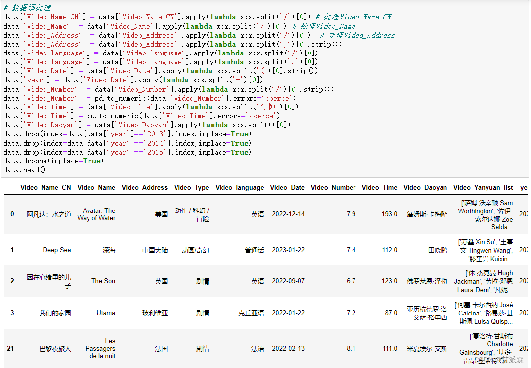
3. Field processing
Since the information in each field in the crawled raw data is very messy, there are many "/" "," and the like, which are processed here in a unified manner, mainly using the apply() function in pandas, and because the data we analyzed in 2016- Movie data in 2023, other than that will be deleted
# 数据预处理
data['Video_Name_CN'] = data['Video_Name_CN'].apply(lambda x:x.split('/')[0]) # 处理Video_Name_CN
data['Video_Name'] = data['Video_Name'].apply(lambda x:x.split('/')[0]) # 处理Video_Name
data['Video_Address'] = data['Video_Address'].apply(lambda x:x.split('/')[0])  # 处理Video_Address
data['Video_Address'] = data['Video_Address'].apply(lambda x:x.split(',')[0].strip())
data['Video_language'] = data['Video_language'].apply(lambda x:x.split('/')[0])
data['Video_language'] = data['Video_language'].apply(lambda x:x.split(',')[0])
data['Video_Date'] = data['Video_Date'].apply(lambda x:x.split('(')[0].strip())
data['year'] = data['Video_Date'].apply(lambda x:x.split('-')[0])
data['Video_Number'] = data['Video_Number'].apply(lambda x:x.split('/')[0].strip())
data['Video_Number'] = pd.to_numeric(data['Video_Number'],errors='coerce')
data['Video_Time'] = data['Video_Time'].apply(lambda x:x.split('分钟')[0])
data['Video_Time'] = pd.to_numeric(data['Video_Time'],errors='coerce')
data['Video_Daoyan'] = data['Video_Daoyan'].apply(lambda x:x.split()[0])
data.drop(index=data[data['year']=='2013'].index,inplace=True)
data.drop(index=data[data['year']=='2014'].index,inplace=True)
data.drop(index=data[data['year']=='2015'].index,inplace=True)
data.dropna(inplace=True)
data.head()
3. Data visualization
1. Import the visualization library
This visualization mainly uses third-party libraries such as matplotlib, seaborn, pyecharts, etc.
import matplotlib.pylab as plt
import seaborn as sns
from pyecharts.charts import *
from pyecharts.faker import Faker
from pyecharts import options as  opts
from pyecharts.globals import ThemeType
plt.rcParams['font.sans-serif'] = ['SimHei'] #解决中文显示
plt.rcParams['axes.unicode_minus'] = False   #解决符号无法显示
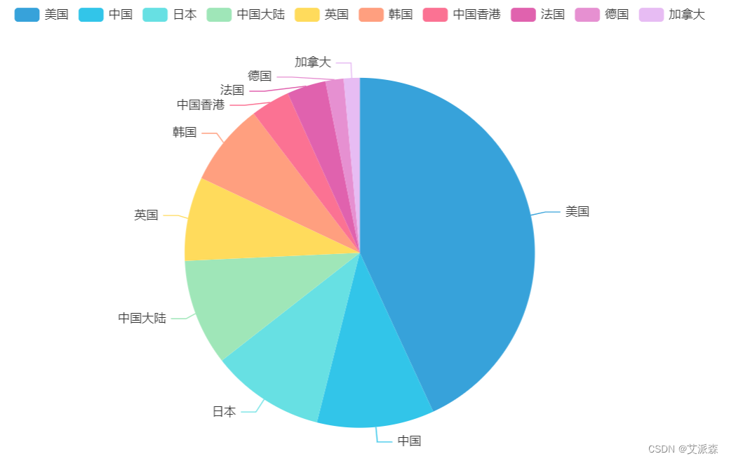
2. Analyze the proportion of movies released in each country
# 分析各个国家发布的电影数量占比
df2 = data.groupby('Video_Address').size().sort_values(ascending=False).head(10)
a1 = Pie(init_opts=opts.InitOpts(theme = ThemeType.LIGHT))
a1.add(series_name='电影数量',
        data_pair=[list(z) for z in zip(df2.index.tolist(),df2.values.tolist())],
        radius='70%',
        )
a1.set_series_opts(tooltip_opts=opts.TooltipOpts(trigger='item'))
a1.render_notebook()
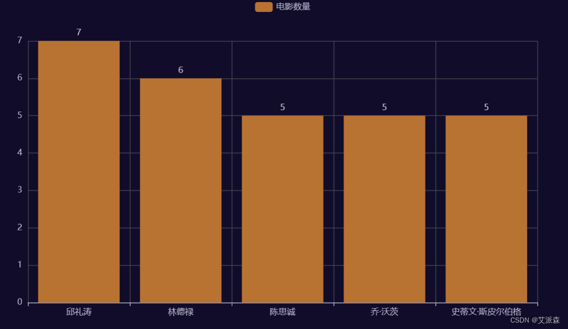
3. Top 5 directors with the highest number of films released
# 发布电影数量最高Top5导演
a2 = Bar(init_opts=opts.InitOpts(theme = ThemeType.DARK))
a2.add_xaxis(data['Video_Daoyan'].value_counts().head().index.tolist())
a2.add_yaxis('电影数量',data['Video_Daoyan'].value_counts().head().values.tolist())
a2.set_series_opts(itemstyle_opts=opts.ItemStyleOpts(color='#B87333'))
a2.set_series_opts(label_opts=opts.LabelOpts(position="top"))
a2.render_notebook()
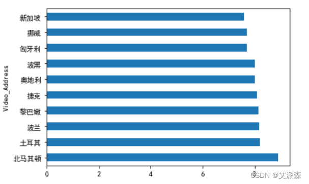
4. Analyze the top ten countries with the highest average film rating
# 分析电影平均评分最高的前十名国家
data.groupby('Video_Address').mean()['Video_Number'].sort_values(ascending=False).head(10).plot(kind='barh')
plt.show()
5. Analyze which language is the most popular
# 分析哪种语言最受欢迎
from pyecharts.charts import WordCloud
import collections
result_list = []
for i in data['Video_language'].values:
    word_list = str(i).split('/')
    for j in word_list:
        result_list.append(j)
result_list
word_counts = collections.Counter(result_list)
# 词频统计:获取前100最高频的词
word_counts_top = word_counts.most_common(100)
wc = WordCloud()
wc.add('',word_counts_top)
wc.render_notebook()

6. Analyze which type of movie is the most popular
# 分析哪种类型电影最受欢迎
from pyecharts.charts import WordCloud
import collections
result_list = []
for i in data['Video_Type'].values:
    word_list = str(i).split('/')
    for j in word_list:
        result_list.append(j)
result_list
word_counts = collections.Counter(result_list)
# 词频统计:获取前100最高频的词
word_counts_top = word_counts.most_common(100)
wc = WordCloud()
wc.add('',word_counts_top)
wc.render_notebook()

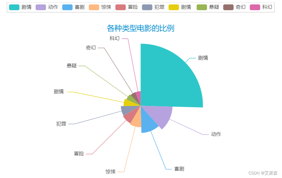
7. Analyze the ratio of various types of movies
# 分析各种类型电影的比例
word_counts_top = word_counts.most_common(10)
a3 = Pie(init_opts=opts.InitOpts(theme = ThemeType.MACARONS))
a3.add(series_name='类型',
        data_pair=word_counts_top,
        rosetype='radius',
        radius='60%',
        )
a3.set_global_opts(title_opts=opts.TitleOpts(title="各种类型电影的比例",
                        pos_left='center',
                    pos_top=50))
a3.set_series_opts(tooltip_opts=opts.TooltipOpts(trigger='item',formatter='{a} <br/>{b}:{c} ({d}%)'))
a3.render_notebook()
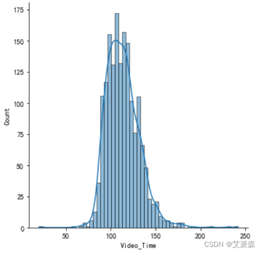
8. Analyze the distribution of movie lengths
# 分析电影片长的分布
sns.displot(data['Video_Time'],kde=True)
plt.show()
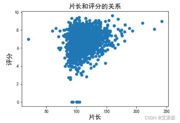
9. Analyze the relationship between film length and rating
# 分析片长和评分的关系
plt.scatter(data['Video_Time'],data['Video_Number'])
plt.title('片长和评分的关系',fontsize=15)
plt.xlabel('片长',fontsize=15)
plt.ylabel('评分',fontsize=15)
plt.show()
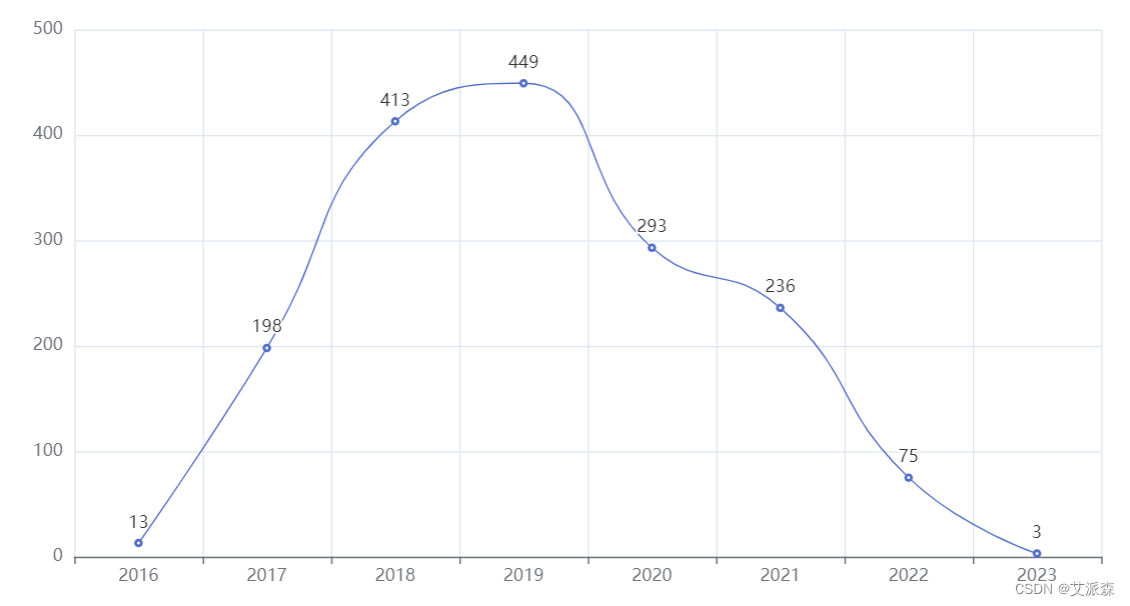
10. Statistics of the total number of movies produced from 2016 to the present
# 统计 2016 年到至今的产出的电影总数量
df1 = data.groupby('year').size()
line = Line()
line.add_xaxis(xaxis_data=df1.index.to_list())
line.add_yaxis('',y_axis=df1.values.tolist(),is_smooth = True)
line.set_global_opts(xaxis_opts=opts.AxisOpts(splitline_opts = opts.SplitLineOpts(is_show=True)))
line.render_notebook()
Four. Summary
This experiment uses crawlers to obtain movie data from 2016 to 2023, and draws the following conclusions through visual analysis:
1. The number of movies gradually increased from 2016 to 2019, reached the maximum in 2019, and began to decline rapidly year by year from 2020.
2. The countries with the largest number of released movies are China and the United States.
3. The feature film with the most movie types.
4. The film length is normally distributed, and the film length and rating are positively correlated.
Welfare at the end of the article
Finally, I would like to thank everyone who has read my article carefully. Reciprocity is always necessary. Although the following information is not very valuable, you can take it away if you need it:
- ① Learning roadmap for all directions of Python, clear what to learn in each direction
- ② More than 600 Python course videos, covering the necessary basics, crawlers and data analysis
- ③ More than 100 practical cases of Python, including detailed explanations of 50 super-large projects, learning is no longer just theory
- ④ 20 mainstream mobile games forced solutions Retrograde forced solution tutorial package for reptile mobile games
- ⑤ Crawler and anti-crawler offensive and defensive tutorial package, including 15 large-scale website forced solutions
- ⑥ Reptile APP reverse actual combat tutorial package, including detailed explanations of 45 top-secret technologies
- ⑦ More than 300 Python e-books, ranging from beginners to advanced
- ⑧ Huawei produces exclusive Python comic tutorials, which can also be learned on mobile phones
- ⑨ The actual Python interview questions of Internet companies over the years are very convenient for review