Author: Night Passerby
Time: April 12, 2023
What is AIGC
AIGC - AI Generated Content (AI Generated Content), corresponding to our past is mainly UGC (User Generated Content) and PGC (Professional user Generated Content).
AIGC means that all output content is generated by AI robots. The main difference is that in the past, ordinary users and professional users (people) in a certain field produced content. AIGC mainly relies on artificial intelligence (non-human) to generate content. , this is the core meaning of AIGC.
(Copyright identification: UGC and PGC have the concept of copyright, and the copyright belongs to the person responsible for generating the content. Currently, AIGC US regulations believe that there is no concept of copyright, that is, the content does not belong to the caller, nor does it belong to the AI machine, so there is no This matter belongs to copyright.)
What content can AIGC generate
At present, AIGC can mainly generate text content and image content (currently there are some products for video generation, but they are not as mature as text and image generation), so we mainly focus on the introduction of AIGC for text and images.
In terms of text content, AIGC can mainly interact in the form of Q&A (question answering), and can produce and output content that meets human expectations according to the "questions" that humans want.
Generally, we can think of AI as an all-knowing and omnipotent "advanced human", using "text AIGC", you can ask it questions (Prompt), and then it will answer accordingly. All questions and answers can involve all aspects, including but not limited to encyclopedia knowledge/creative copywriting/novel script/code programming/translation conversion/thesis writing/education and teaching/guidance advice/chat companionship, etc. You need to think about it all, and you can understand that it is a "baixiaosheng" with knowledge of the whole earth, and you can ask it or communicate with it about anything.
For example, we use the famous ChatGPT to ask questions:

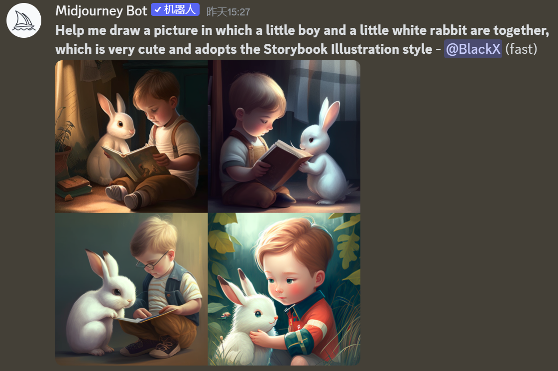
For "Picture AIGC", you may have countless ideas in your mind, but you can't paint, and you can't turn the Ideas in your mind into real pictures. Then, "Picture AIGC" can help you follow what you want in your mind. You tell it what you want, and then it can help you draw it for you in the form of picture painting, allowing you to turn your "creativity" into picture reality at once.
For example, we use the very useful "picture AIGC" tool Midjourney to draw:
Basic working principle of AIGC
The bottom layer of AIGC mainly relies on AI technology. The essence of AI technology is to enable machines to have the same intelligence as humans (Artificial Intelligence), so it is necessary to allow machines to learn and think like humans. Therefore, most of the underlying technologies that implement AI are called artificial intelligence. "Machine Learning" (Machine Learnin) technology.
There are many application scenarios for machine learning technology. For example, face recognition (mobile phone unlocking/Alipay payment/access control unlocking, etc.), speech recognition (Xiaoai classmates/Xiaodu/Siri), face-changing (anchor beauty, etc.) are very commonly used now. beauty/beauty camera), map navigation, weather forecast, search engine, NLP (Natural Language Processing), automatic driving, robot control, AIGC, etc.
Today I will focus on learning about the image generation technology in AIGC, that is, the AIGC of images. At present, mainstream image AIGC products at home and abroad include OpenAI DALL.E, Google Imagen, Stable Diffusion, MidJourney, Disco Diffusion and so on. At present, the mainstream applications are widely used mainly including Stable Diffusion and MidJourney products. The working principles of these products are similar. The following mainly takes the Stable Diffusion product as an example to briefly learn the main technical principles of the underlying technology of AI image generation.
How Machines Learn
Machine learning can be simply understood as the process of simulating human learning. Let's take a look at how machines simulate human learning.
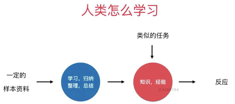
Let's look at the so-called "machine learning":

For human learning, the things we see and encounter are our "data" (corpus), and then we pass "learning summary" (learning algorithm), and finally become "knowledge experience wisdom" (model ), and when we encounter something, we will call these "knowledge experience methodology" to make corresponding response decision-making actions (predictive reasoning);
For machine learning, a large amount of "corpus" is input to it (seeing things encountered), and then through machine learning algorithms (summarization and induction to extract similar points), and finally a "model" (knowledge experience methodology) is formed, and then When encountering some decisions that need to be judged, we will give the "model" the things to be judged and decided, and then tell us the output results (reasoning and speculation results);
From the abstraction level, we will find that, in essence, the intrinsic nature of "human learning" and "machine learning" is quite similar.
Let's take a look at the process of machine learning in a computer:
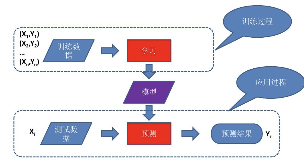
The core steps are: "training data ➜ training algorithm ➜ model ➜ prediction ➜ output results", where the final output is the "model" (Model, model file), and then mainly the pre-"training model" and the post- "Model prediction", and then generate corresponding results.
We can simply understand the above process as: the "model" is a puppy, and the breeder is the "training algorithm". The puppy will learn some skills (models). Once learned, the puppy can go out to perform, and the process of performance is prediction.
So we will see that if there are more features (knowledge experience) in the "model", it will be more accurate in the "prediction" stage. If the model is smaller, or the feature data in the middle is less, the accuracy of the final prediction result may be higher. will decrease. (Similarly, the more things a person encounters, the more experience he can sum up. As the saying goes, "There are no white roads and no white pits in life" is probably this logic)
Image generation core model - Diffusion Model
In the field of image generation, there have been four mainstream generative models in recent years: generative adversarial model (GAN), variational autoencoder (VAE), flow model (Flow based Model), diffusion model (Diffusion Model), etc., basically It is mainly a model based on deep learning as a training method. Starting from 2022, the main popular image generation model is the Diffusion Model (diffusion model).
(Comparison diagram of several mainstream image processing models)

At present, mainstream reliable image generation technologies at home and abroad are basically implemented based on the Diffusion Model, including but not limited to Stable Diffusion, MidJourney, OpenAI DALL.E, Disco Diffusion, Google Imagen and other mainstream products, but the actual The technology is different in terms of processing, which also leads to different forms of expression. The core is that the underlying model training image corpus is different, and the other is the fine-tuning of some algorithms.
Diffusion uses an unsteady-state generative model, the core of which is a generative model that expects good results by constantly removing noise. The early diffusion model did not work well in AI painting, and it took 10-15 minutes to generate a single image. Later, a British company called Stability AI improved the model, greatly improving the stability and quality of image generation, and the image generation speed It has been increased by 100 times, which means that it used to take 10-15 minutes (600-900 seconds) and now it only takes 6-10 seconds to generate a picture (I personally measured that it takes about 10 seconds to generate a picture under the RTX4050-6G graphics card. about). Then the company called this steady-state Diffusion model: "Stable Diffusion", and the shape of the Stable Diffusion model has basically influenced AI art painting products such as MidJourney.
Before the emergence of Stable Diffusion (stable diffusion model), there was a stable diffusion model (Latent Diffusion). Latent diffusion is actually the text2image model in the Latent diffusion paper. Latent diffusion is more precisely a Latent-based diffusion model. Architecture, so Stable Diffusion also belongs to Latent Diffusion in essence, because the company behind Stable Diffusion developing this model is called Stability Al, so it is called Stable Diffusion.
Of course, Stable Diffusion still has many improvements. Compared with Latent Diffusion, the main improvements of Stable Diffusion include:
(1) Training data: Latent diffusion% is trained on laion-400M data, while Stable diffusion is trained on laion-2B.en data set, obviously the latter uses more training data, and the latter also uses Data filtering is performed to improve data quality, such as removing images with watermarks and selecting images with higher aesthetic scores.
(2) text-encoder: Latent diffusion uses a randomly initialized transformer to encode text, while Stable diffusion uses a pre-trained CLIP text encoder to encode text. The pre-trained text model is often better than the model trained from scratch
(3) Training size: Latent diffusion is only trained on 256x256 resolution, while Stable diffusion is pre-trained on 256x256 resolution first, and then Finetune on 512x512 resolution.
To sum up: Stable diffusion uses a better text encoder to train on a larger data set and can generate higher-resolution images, so Stable Diffusion is more suitable for practical applications in image generation.
Let's have a brief understanding of Stable Diffusion. Its main algorithm working structure is roughly like this:

The core architecture diagram in the middle is the diagram in the reference paper " High-Resolution Image Synthesis with Latent Diffusion Models ". I added a dotted frame outside to mark the core modules.
Stable Diffusion usage workflow
Let's take a look at the basic user operation interaction process of the picture AIGC:
Enter the prompt word (Prompt) -> click "Generate" (or execute the command imagine) -> refresh the picture from 10% to 100% (from blurry to clear) -> the picture is completely generated.
The steps of generating pictures from detailed text can be simply seen as the following steps:
The first step, Prompt Encoder process (Text Encoder)
The model takes the random seed of the latent space and the text prompt (Prompt) as input at the same time, and then uses the seed of the latent space to generate a random latent image representation with a size of 64×64, and converts the input text prompt to a size of for 77×768 text embeddings.
The second step is to use U-Net for the Diffusion process
Using a modified U-Net with an attention mechanism, iteratively denoises random latent image representations while accepting text embeddings as objects of attention computation. The output of U-Net is the residual of the noise, which is used to calculate the denoised latent image representation by the scheduler program algorithm. The scheduler algorithm computes a predicted denoised image representation based on the previous noise representation and the predicted noise residual. The denoising process is repeated about 50-100 times, which allows progressively better latent image representations to be retrieved.
Many different scheduler algorithms can be used for this calculation, each with its advantages and disadvantages. For Stable Diffusion, you can use PNDM scheduler, DDIM scheduler+PLMS, K-LMS scheduler, etc.
In the third step, the latent image is decoded by VAE
Once the above steps are completed, the latent image representation is decoded by the decoder part of the variational autoencoder, outputting the picture, and the step is completed.
(The main workflow flow chart of the above three steps)

The underlying working mechanism of Stable Diffusion
Let's sort out the above usage process. These steps can be sorted out. The core operation process is mainly these three steps, and then mapped into our corresponding modules as:
Step 1. Enter the prompt words and parse the prompt words: Text Image Encoder - CLIP
Step 2. Pull a model suitable for prompt words from the image library (model): Diffusion process based on U-Net (DDPM+DDIM+PLMS based on U-Net)
Step 3. Processing and conversion of image input and output: VAE
If these three core steps are involved, then these algorithm models with English capital letters mainly depend on them, etc. Let us briefly introduce:
(1) Text Encoder: CLIP - Contrastive Language-Image Pre-training
is a pre-training method or model based on contrastive text-image pairs, and CLIP is a multimodal model based on contrastive learning. The training data of CLIP is a text-image pair, mainly an image and its corresponding text description. It is hoped that through comparative learning, the model can learn the matching relationship between the text-image pair.
The full English name of CLIP is Contrastive Language-Image Pre-training, which is a pre-training method or model based on contrastive text-image pairs. It is easier to collect a large number of pairs of text and images on the Internet. For any image-text pair, the text can actually be regarded as the label of the image. CLIP is a multimodal model (text + image) based on contrastive learning. Unlike some comparative learning methods in CV such as moco and simclr, the training data of CLIP is a text-image pair: an image and its corresponding The text description, here hope that through contrastive learning, the model can learn the matching relationship between text-image pairs. As shown in the figure below, CLIP includes two models: Text Encoder and Image Encoder. Text Encoder is used to extract text features, and the text transformer model commonly used in NLP can be used; Image Encoder is used to extract image features. Commonly used CNN model or vision transformer. (To put it simply: it is to put text and pictures into a matrix space, which is used to solve the mapping and similarity intersection of text to pictures, so that it is convenient to find the distribution model of corresponding images through text)
(Working process of CLIP)
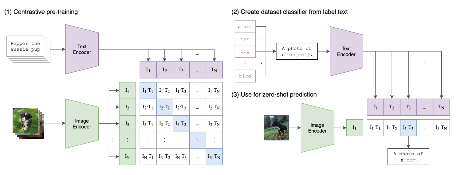
Let's look at the above picture, we observe the process of Contrastive pre-training, where the extracted text features and image features are compared and learned. For a training batch containing N text-image pairs, combining N text features and N image features in pairs, the CLIP model will predict the similarity of N^2 possible text-image pairs, where the similarity Directly calculate the cosine similarity (cosine similarity) of text features and image features, which is the matrix shown in the figure above. There are a total of N positive samples, that is, the text and image that really belong to a pair (diagonal elements in the matrix), and the remaining N^2 - N text-image pairs are negative samples, then the training goal of CLIP is the largest The similarity of N positive samples, while minimizing the similarity of N^2 - N negative samples, this is the working principle of the general training process.
(2) Image generation process: UNet-based Diffusion Process (DDPM, etc.)
This is the most complex and critical process in image AIGC. The main thing to solve is to synthesize the original image according to the abstract image distribution model or noise. Taking Stable Diffusion as an example, it is mainly based on the idea of Diffusion Model, including DDPM (Denoising Diffusion Probabilistic Models, denoising diffusion probability model). DDPM learns the process of denoising by continuously adding noise to the data to become real noise, and continuously denoising and restoring the original data from the real noise, and then can randomly sample the real noise and restore (generate) it into each All kinds of data.
As the most critical process, simply speaking, the whole idea of the diffusion model (Diffusion Model) is simply to add noise to the image continuously to destroy the image, and then continuously denoise the damaged image, and finally restore the original image. DDPM is an implementation of a Diffusion model, which uses a special distribution that is gradually "sampled" from Gaussian noise according to certain conditions, and the generated pictures/voices are finally obtained as the number of "sampling" rounds increases. In other words, the synthesis process of the Diffusion Model is to extract the required image/audio from the noise through iterations. As the number of iterations increases, the synthesis quality is getting better and better.
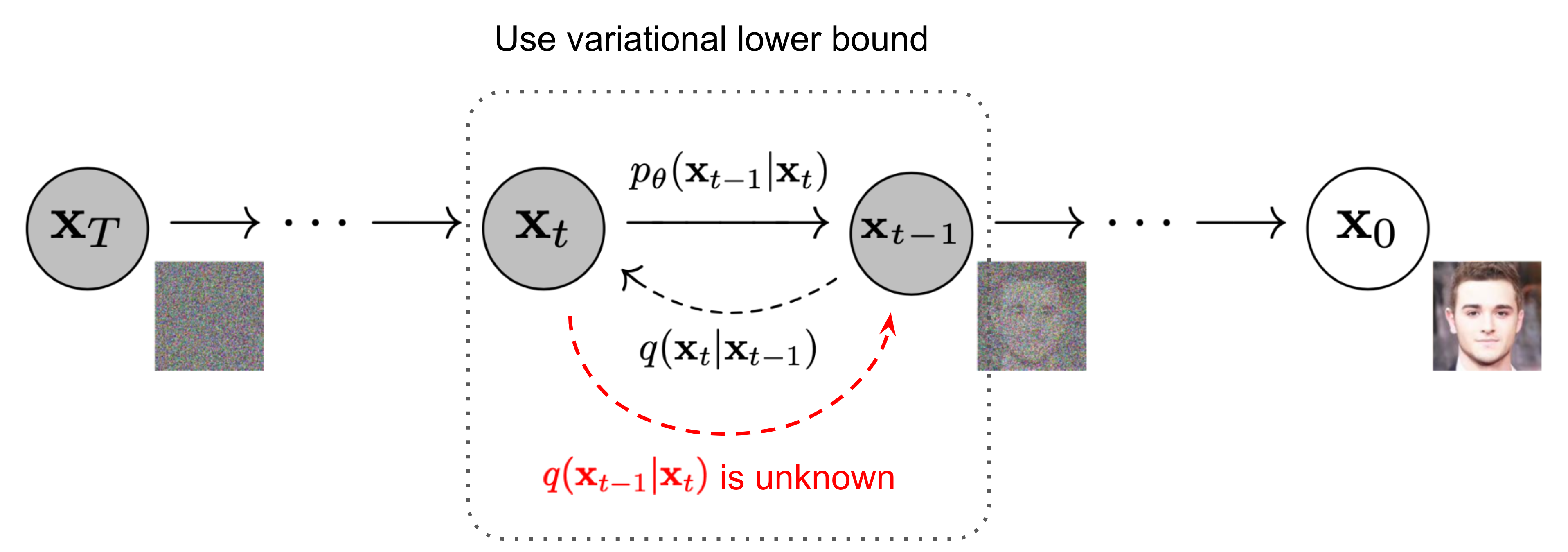
Diffusion model includes two processes: forward process (forward process) and reverse process (reverse process reverse process), where the forward process is also called the diffusion process (diffusion process), whether it is a forward process or a reverse process A parameterized Markov chain (Markov chain), where the reverse process can be used to generate data, here we will be modeled and solved by variational inference.
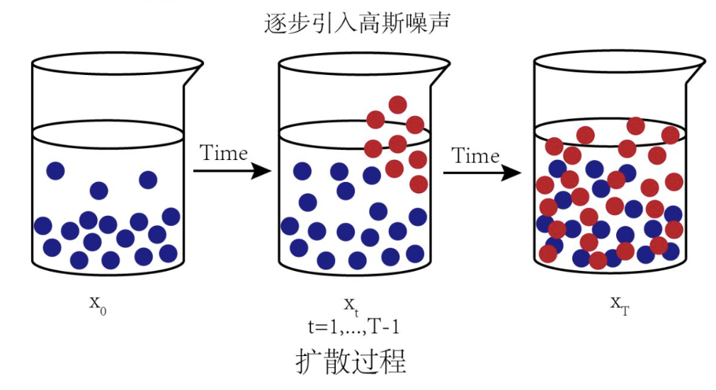
The diffusion process (forward process) refers to the process of gradually adding Gaussian noise to the data until the data becomes random noise.
The diffusion process is to noise the data, then the reverse process is a denoising process, if we know the true distribution of each step of the reverse process, then starting from a random noise, gradually denoising can generate a real sample, So the reverse process is the process of generating data.
Then the core of the diffusion model is to train the noise prediction model. Since the noise and the original data are of the same dimension, we can choose to use the AutoEncoder architecture as the noise prediction model. The model adopted by DDPM is a U-Net model based on residual block and attention block.
The whole diffusion process refers to the process of gradually adding Gaussian noise to the data until the data becomes random noise. For the diffusion model, we often call the variance of different steps the variance schedule or noise schedule. Usually, the later step will use a larger variance. Under a well-designed variance schedule, if the number of diffusion steps is sufficient Large, then the final result completely loses the original data and becomes a random noise. Each step of the diffusion process generates a noisy data, and the entire diffusion process is a Markav chain. The diffusion process is often fixed, that is, a pre-defined variance schedule is adopted. For example, DDPM adopts a linear variance schedule.
(Forward and reverse process of Diffusion Model)
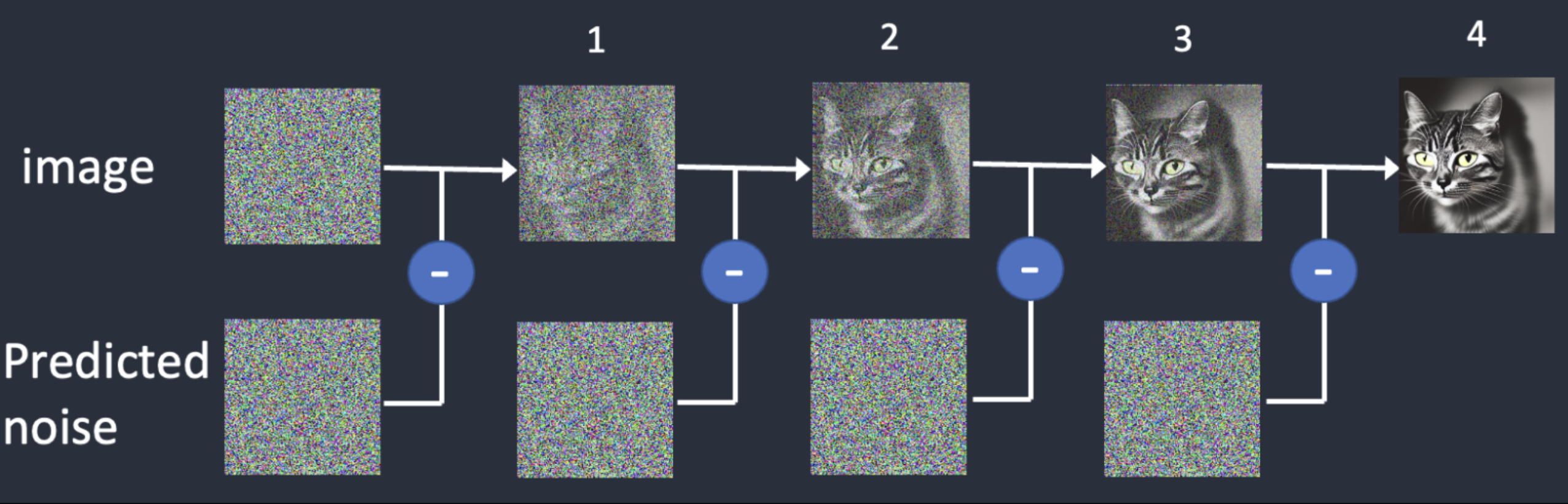
The big process of the diffusion model lies in the sampling of noise. Model sampling needs to start from a pure noise picture, denoise it step by step, and finally get a clear picture. In this process, the model must serially calculate at least 50 to 100 steps to obtain a higher quality picture, which leads to the time required to generate a picture 50 to 100 times that of other deep generative models, which greatly limits the model deployment and landing.
These sampling processes are mainly mapped to the Scheduler in the Stable Diffusion program. The main function of the Scheduler in Stable Diffusion is to output the coefficient of the generated image noise according to the current step of the generated noise. It is simple to calculate. The formula is: (image noise = randomly generated noise * coefficient of scheduler output). The scheduler will accept parameters including the step of the current generated noise as input when calculating the coefficients, and then generate and return the corresponding coefficients.
Under the driving requirements of sampling frequency and speed, the diffusion model is very important for noise addition and denoising sampling schemes. There are many types in the new and old, and the key is the sampling process, including PNDM, DDIM, PLMS, K-LMS , DPM-Solver, etc. From the perspective of the latest version, the main sampling methods include DDPM, DDIM, PLMS, and DPM-Solver.
DDPM (Denoising Diffusion Probabilistic Model), because the traditional "diffusion model" uses the Langevin equation to sample from the energy model, there is also great uncertainty, and the obtained sampling results are often noisy. So for a long time, the diffusion model of this traditional path was only experimented on relatively low-resolution images. The DDPM (Denoising Diffusion Probabilistic Model) proposed in 2020 is a new starting point and a new chapter. It is more accurate to call DDPM "Gradient Diffusion Model". The mathematical framework of DDPM has been completed in ICML2015 paper "Deep Unsupervised Learning using Nonequilibrium Thermodynamics", but DDPM is the first time to debug it on high-resolution image generation. , which leads to the hotness of the subsequent picture generation. DDPM uses a linear noise-adding sampling scheme (linear schedule) by default.
PNDM is a new numerical method suitable for diffusion models. This method does not require retraining the model, and has no additional restrictions on the model structure and hyperparameters. Only by modifying the iteration formula, the diffusion model can be accelerated without any loss of accuracy. 20 times, the FID result of the original 1000 steps can be achieved after 50 iterations.
DDIM (Denoising Diffusion Implicit Models, denoising diffusion implicit model), DDIM and DDPM have the same training objectives, but it no longer restricts the diffusion process to be a Markov chain, which allows DDIM to use smaller sampling steps To speed up the generation process, another feature of DDIM is that the process of generating samples from a random noise is a deterministic process.
PLMS (Pseudo Linear Multi-Step method, pseudo-linear multi-step method) is mainly based on the principle of the diffusion model to sample the next step of the picture, mainly to gradually reconstruct the reverse denoising process of the picture, and apply the corresponding updated diffusion for each step of the picture Each parameter of the process generates the next picture, which is mainly a linear sampling method.
DPM-Solver (Diffusion Process Model Solver) is proposed by the TSAIL team led by Professor Zhu Jun of Tsinghua University. It is an efficient solver specially designed for diffusion models: the algorithm does not require any additional training and is applicable to For both discrete-time and continuous-time diffusion models, convergence can be nearly achieved in 20 to 25 steps, and very high quality sampling can be obtained in only 10 to 15 steps. On Stable Diffusion, 25-step DPM-Solver can obtain better sampling quality than 50-step PNDM, so the sampling speed is directly doubled.
(3) Image generation training network: UNet (U-shaped neural network training model)
From the above content, we know that the core of the diffusion model is to train the noise prediction model. Since the noise and the original data are of the same dimension, Stable Diffusion chooses the AutoEncoder architecture as the noise prediction model. The model adopted by DDPM is a U-Net model based on residual block and attention block.
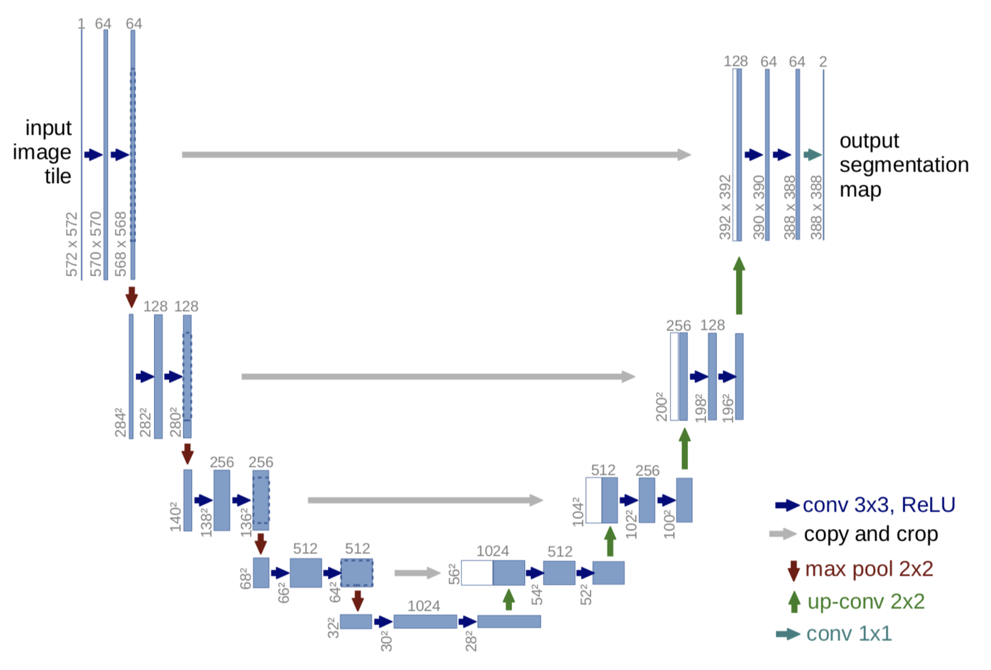
U-Net belongs to the encoder-decoder architecture, in which the encoder is divided into different stages, each stage contains a downsampling module to reduce the space size of the feature (H and W), and then the decoder is the opposite of the encoder, and gradually restores the features compressed by the encoder. . U-Net also introduces skip connection in the decoder module, that is, concats the same-dimensional features obtained in the middle of the encoder, which is conducive to network optimization. Each stage of U-Net used by DDPM contains 2 residual blocks, and some stages also add a self-attention module to increase the global modeling capability of the network. In addition, the diffusion model actually needs T noise prediction models. In actual processing, we can add a time embedding (similar to the position embedding in the transformer) to encode the timestep into the network, so that only one shared U-Net needs to be trained Model. Specifically, DDPM introduces time embedding in each residual block.
(The U-Net model is used in the training of the forward diffusion process, the middle purple part)

Unet is a model proposed in "U-Net: Convolutional Networks for Biomedical Image Segmentation" in 2015. UNet is a semantic segmentation model. Its main execution process is similar to other semantic segmentation models. First, convolution is used for downsampling, and then layer-by-layer features are extracted. Using this layer-by-layer feature, it performs Upsampling, and finally an image with each pixel corresponding to its type. The feature map obtained by the deeper the network layer in Unet has a larger field of view. The shallow convolution focuses on the texture features, and the deep network focuses on the essential features, so the deep and shallow features have a grid meaning; another point It is the edge of a larger-sized feature map obtained through deconvolution, which lacks information. After all, every time downsampling extracts features, it will inevitably lose some edge features, and the lost features cannot be obtained from upsampling. Retrieval, so through the splicing of features, a retrieval of edge features is realized.
(Working structure of U-Net)
Unet is the most commonly used and relatively simple segmentation model. It is simple, efficient, easy to understand, easy to build, and can be trained from small data sets. It is very simple and easy to use in Diffusion Model.
(4) Input and output image codec: VAE (Variational Auto Encoder, Variational Auto Encoder)
VAE consists of two parts: Encoder and Decoder. The encoder is used to convert the image into a low-dimensional latent representation, which will be used as input to the U-Net model. Instead, the decoder converts the latent data representation back into an image.
During Latent Diffusion Model training, the Encoder is used to obtain a latent representation of the image in the forward diffusion process, applying more and more noise at each step. In the inference process, the denoising latent generated in the back-diffusion process is converted back to the image through the VAE Decoder, and only the VAE Decoder is needed in the actual inference process.
(The process of VAE in the Diffusion Process)

VAE is also a form of deep generative model, which is a generative network structure based on Variational Bayesian (VB, Variational Bayes) inference proposed by Kingma in 2014. Different from the traditional autoencoder which describes the latent space numerically, it describes the observation of the latent space probabilistically, showing great application value in data generation. As soon as VAE was proposed, it quickly gained widespread attention in the field of deep generative models, and it is regarded as one of the most research-worthy methods in the field of unsupervised learning together with Generative Adversarial Networks (GAN). More and more applications.
Autoencoder (AE, Auto Encoder), autoencoder is an unsupervised learning method, its principle is very simple: first map the high-dimensional original data to a low-dimensional feature space, and then learn from the low-dimensional features to reconstruct the original The data. An AE model consists of two parts of the network. Including Encoder, which mainly maps the original high-dimensional data to a low-dimensional feature space. This feature dimension is generally smaller than the original data dimension, so as to achieve the purpose of compression or dimensionality reduction. This low-dimensional feature often becomes an intermediate hidden feature. Features (latent representation) and Decoder, based on the compressed low-dimensional features to reconstruct the original data.
Although VAE (Variational Auto Encoder) also has Auto Encoder in its name, this is mainly because VAE and AE have a similar structure, that is, the architecture design of encoder and decoder. In fact, there is a big difference between VAE and AE in terms of modeling. In essence, VAE is a probabilistic model (Probabilistic Model) based on variational inference (Variational Inference, Variational Bayesian methods), which belongs to the generative model ( And of course an unsupervised model). On the basis of Autoencoder (AE), VAE makes the potential vector of image encoding obey Gaussian distribution to realize image generation, optimizes the lower bound of data logarithmic likelihood, VAE can be parallelized in image generation, and the speed is improved, but VAE also has the problem of generating image blur.
(VAE core working principle)

The underlying mathematical principles of Diffusion Model
The core idea of Diffusion Model is:
First, noise is continuously added to the training data, and then the signal is gradually recovered from the noise in the reverse process. It is fundamentally different from other generative models;
Diffusion Model splits the image generation process into N (eg N=1000) small "denoising" steps. The model gradually removes noise through these "small steps", accumulating small victories into big victories, and finally generating high-quality Sample .
The diffusion model of the whole idea of DDPM is inspired by the hidden variable model inspired by non-equilibrium thermodynamics (in non-equilibrium thermodynamics, the solution of the Langevin equation can obtain the "fluctuation-dissipation relationship"), and a diffusion is defined in the Diffusion Model Markov chain of steps (the current state is only related to the state at the previous moment), slowly adding random noise to the real data (forward process), and then learning the reverse diffusion process (inverse diffusion process), from the noise Build the required data samples.

Looking at the figure above, the forward process of the diffusion model does not contain learnable parameters. As t increases, the final distribution becomes an independent Gaussian distribution in all directions. We gradually add a small Gaussian noise in the forward pass for a total of T steps, resulting in a series of noised samples.
Diffusion first appeared in ICML2015's paper "Deep Unsupervised Learning using Nonequilibrium Thermodynamics". At that time, the author completed the overall framework and mathematical derivation formula, but the real task of cv and nlp was DDPM, which was the first time to generate it in high-resolution images. On debugging, it is highly compatible with the UNet network, allowing everyone to see the potential of Diffusion in vision. At present, the model has gradually expanded to nlp, RL, ML and other fields, but it is mainly in the field of image generation, including ours. Stable Diffusion, MidJourney, OpenAI DALL.E, Disco Diffusion, Google Imagen and other image generation products mentioned above.
Diffusion Model's underlying mathematical and physical theory is mainly supported by "Markov Chain", Langevin equation (Langevin equation), and Gaussian distribution (Gaussian Distribution, normal distribution) and KL scattered value and other basic formula principles.
The process of image generation can be mainly understood as the process of removing noise and deriving it into the original picture. In the process of adding noise to the picture, it is similar to the transfer of substances from high-concentration areas to low-concentration areas in non-equilibrium thermodynamics until they are evenly distributed; similar to that in a glass of water. A drop of pigment is added to the water, and then the entire pigment will gradually spread throughout the clear water in a manner similar to Brownian movement, and finally it will look evenly distributed. (Langevin equation)


The process of making the picture blurred and modeling can be understood as that the next picture of each picture is a little bit blurrier than the previous one (noise conforming to the Gaussian distribution), and then each picture becomes the next one mainly depends on the previous picture. one sheet. (Markov chain)

In the inverse diffusion process, the Markov process is represented as consisting of cumulative transformations under a continuous conditional Gaussian distribution. With the overall optimization strategy, it depends on the calculation method of each pixel. At the end of the inverse diffusion process, we hope to get a generated image, so we need to design a method so that each pixel value on the image satisfies Discrete log-likelihood, so will be combined with KL divergence below the synchronous Gaussian distribution.
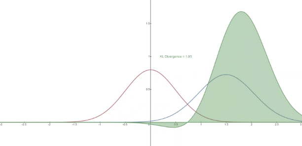
KL divergence is an asymmetric statistical distance measure used to measure the degree of difference between one probability distribution P and another probability distribution Q. The reason why the Diffusion Model wants to solve it according to the KL divergence
, because according to the definition of Diffusion Models, the transition distribution in the Markov chain belongs to Gaussian distribution, and KL divergence can be used to calculate the difference distance between two Gaussian distributions. All KL divergences are now compared between Gaussian probability distributions, which means that closure expressions can be used to compute exact variational upper bounds instead of sampled Monte Carlo estimation.
(1) Langevin equation
The Langevin equation (Langevin formula) is a description of stochastic differential equations describing the time evolution of a subset of degrees of freedom discovered by the French physicist Paul Langevin in 1908, mainly describing the Brownian motion The process; that is, due to the collision with the fluid molecules, the average moving position of the Brownian motion particles is proportional to the square of the distance from the origin (initial point) and the time. It is an intuitive explanation for the diffusion motion. As time goes by, the particles run more and more "scattered".
Through the Langevin equation, we can obtain the distribution of particles. By simulating dynamics to sample the distribution, we can accurately simulate the movement of particles in potential energy and thermal fluctuations, capture the position of the particles, and use them as samples to obtain the desired distribution. (Boltzmann distribution). Simply put, the sampling process can be accelerated using Langevin kinetics.
In addition to the mathematical principles of Diffusion Model, in fact, each module involves various related underlying mathematical models and algorithm principles, so I will not introduce them one by one.
(2) Gaussian Distribution (Gaussian Distribution, normal distribution)
Gaussian Distribution (Gaussian Distribution), also known as Normal Distribution (Normal Distribution), also known as normal distribution, is a common continuous probability distribution.
The concept of normal distribution (Gaussian distribution) was first proposed by the French mathematician Abraham de Moivre in 1733. He discovered it in the asymptotic formula for the binomial distribution, and later by the German mathematician Gauss (Johann Carl Friedrich Gauss) derived it from another angle when studying measurement error. Gauss's work had a great influence on later generations. He gave the normal distribution the name "Gaussian distribution" at the same time. The normal distribution (Gaussian distribution) is a very important probability distribution in the fields of mathematics, physics and engineering, and has a great influence in many aspects of statistics. Gaussian distribution is known as "God's distribution". Its powerful modeling ability and beautiful mathematical properties make Gaussian distribution widely used in reality.

In the diffusion process and inverse diffusion process of Diffusion Models, that is, in the diffusion process, a little noise is artificially added until the data is pure Gaussian noise; the inverse diffusion process learns the reversed distribution and gradually restores the sample data.
In the inverse diffusion process, the Markov process is represented as consisting of cumulative transformations under a continuous conditional Gaussian distribution. With the overall optimization strategy, it depends on the calculation method of each pixel. At the end of the inverse diffusion process, we hope to get a generated image, so we need to design a method so that each pixel value on the image satisfies Discrete log-likelihood, so will be combined with KL divergence below the synchronous Gaussian distribution.
KL divergence is an asymmetric statistical distance measure used to measure the degree of difference between one probability distribution P and another probability distribution Q. The reason why the Diffusion Model wants to solve it according to the KL divergence
, because according to the definition of Diffusion Models, the transition distribution in the Markov chain belongs to Gaussian distribution, and KL divergence can be used to calculate the difference distance between two Gaussian distributions. All KL divergences are now compared between Gaussian probability distributions, which means that closure expressions can be used to compute exact variational upper bounds instead of sampled Monte Carlo estimation.
(3) Markov Chain (Markov Chain, Markov Model)
"Markov chain" is a general law model that can explain natural changes by mathematical methods researched and proposed by Russian mathematician Andrey Andreyevich Markov, named Markov chain. Markov Chain. The Markov chain is a random process of transition from one state to another in the state space. This process requires "no memory", that is, the probability distribution of the next state can only be determined by the current state. In the time series The events before it have nothing to do with it, and the Markov chain believes that all the information in the past has been preserved in the current state. The application of Markov chain in machine learning, natural speech processing research allows machines to "understand" human language, and the Markov model solves it. For example, the acoustic model uses HMM (Hidden Markov Model, invisible Markov model) Modeling, such as the language model N-Gram, which assumes that the appearance of the nth word is only related to the previous N-1 words, and not related to any other words. The probability of the entire sentence is the product of the probability of each word.

Mathematically understand the Markov chain is: a discrete-time random process with Markov properties in mathematics. Describes a sequence of states whose value depends only on the finite number of states preceding it, and has nothing to do with the state before it. You can understand the Markov chain in plain language. For example, if someone failed in the past and gave up on himself, if you use the chicken soup of the Markov chain to tell the other party: "Your future is only related to your present, not to your past. Therefore, Don't worry about how failed you were, start now, it will definitely change (determine) your future."


Simple conclusion of Stable Diffusion principle
Diffusion Model is different from the mechanism of common generative models such as GAN, VAE, and Flow in the past. Denoising Diffusion Probabilistic Model (hereinafter referred to as Diffusion Model) is no longer an input through a "restriction" (such as type, style, etc.), and gradually Add information and finally get the generated picture/voice. Instead, a special distribution is gradually "sampled" from Gaussian noise according to certain conditions, and the generated pictures/voices are finally obtained as the number of "sampling" rounds increases. In other words, the synthesis process of the Diffusion Model is to extract the required image/audio from the noise through iterations. As the number of iterations increases, the synthesis quality is getting better and better.
The benefits of this mechanism are obvious, the quality of synthesis and the speed of synthesis become controllable. When time is sufficient, high-quality synthetic samples can be obtained through high-round iterations, and at the same time, synthetic samples without obvious defects can also be obtained through rapid synthesis in lower rounds. There is no need to retrain the model between high and low rounds of iterations, and only some round-related parameters need to be manually adjusted.
This sounds a bit unbelievable, but there is a strong mathematical logic behind it. These mathematics are mainly the Markov chain and Langevin formula mentioned above. Really, it can only be said that basic mathematics and physics are too powerful.
Regardless of the applied Diffusion Model or the Unet network, the key ideas in it are basically models proposed after 2014-2015, and then shine in the field of image generation models, especially after 2022, various images based on Diffusion Model The resulting products are all brilliant, and excellent products such as Midjourney and Stable Diffusion have emerged.
Any of the above knowledge alone is N papers, just a very brief introduction to the realization principle behind the picture AIGC, knowing it is easy to know why, as an index entry for in-depth learning. It can be considered that Stable Diffusion and other products are basically the masters of various mathematics and deep learning in the past. Standing on the shoulders of giants, the integration of various technologies has produced such excellent image AIGC products.
The above is just a brief overview to understand the principle of AIGC technology outline of the image of the Diffusion Model. Finally, it is simply summarized in the words of scientists. Gauss said: " Mathematics is the king of science ", and Coulter said: " Mathematics is the most brilliant jewel in the crown of human wisdom ".
If you want to know more details, you can refer to related papers and open source codes. There are no secrets in front of papers and source codes.
You can refer to the papers that implement the main algorithm model:
Latent Diffusion:https://arxiv.org/abs/2112.10752
Diffusion:https://arxiv.org/abs/1503.03585
PNDM:https://arxiv.org/abs/2202.09778
DDPM:https://arxiv.org/abs/2006.11239
CLIP:https://arxiv.org/abs/2103.00020
VAE:https://arxiv.org/abs/1312.6114
Some open source code and data for reference:
https://github.com/openai/CLIP
https://github.com/mlfoundations/open_clip
GitHub - Stability-AI/stablediffusion: High-Resolution Image Synthesis with Latent Diffusion Models