Residual Networks (ResNet) - Deep Learning (Residual Networks (ResNet) - Deep Learning)

After the first CNN-based architecture (AlexNet) won the ImageNet 2012 competition, each subsequent winning architecture used more layers in the deep neural network to reduce the error rate. This works fine for fewer layers, but as we increase the number of layers, a common problem in deep learning occurs called vanishing/exploding gradients. This can cause gradients to become 0 or too large. Therefore, when we increase the number of layers, the training and testing error rates also increase.

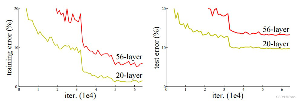
In the figure above, we can observe that the 56-layer CNN has a higher error rate than the 20-layer CNN architecture on both the training and test datasets. Through further analysis of the error rate, it is concluded that the error rate is caused by gradient disappearance/explosion.

ResNet was proposed by researchers at Microsoft Research in 2015, introducing a new architecture called residual network.

1. Residual network

To solve the problem of vanishing/exploding gradients, the architecture introduces the concept of residual blocks. In this network, we use a technique called skip connections. Skip connections connect the activations of one layer to other layers by skipping some layers in between. This forms a stub. Resnets are formed by stacking these remaining blocks together.

The approach behind this network is not to have layers learn the underlying mapping, but to allow the network to fit a residual mapping. So we don't use the H(x) initial mapping and let the network fit.

F(x) := H(x) - x which gives H(x) := F(x) + x.

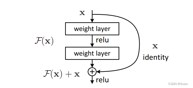
The advantage of adding this type of skip connection is that if any layer hurts the performance of the architecture, it will be skipped by regularization. So this can train a very deep neural network without problems caused by vanishing/exploding gradients. The author of this paper conducted experiments on layers 100-1000 of the CIFAR-10 dataset.

There is a similar method called "highway nets", these nets are also connected by jumper wires. Similar to LSTMs, these skip connections also use parametric gates. These gates determine how much information passes through the skip connections. However, this architecture does not provide better accuracy than the ResNet architecture.

2. Network Architecture

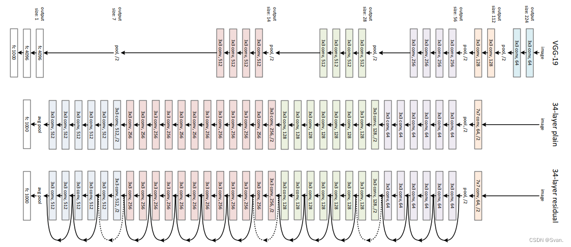
The network adopts a 34-layer flat network architecture inspired by VGG-19, and adds shortcut connections. These shortcut connections then transform the architecture into a residual network.

3. Code running

Using Tensorflow and Keras API, we can design a ResNet architecture (including residual blocks) from scratch. Below are implementations of different ResNet architectures. For this implementation, we use the CIFAR-10 dataset. The dataset contains 60,000 32×32 color images of 10 different categories (airplane, car, bird, cat, deer, dog, frog, horse, boat, and truck), among others. This dataset can be evaluated by keras. datasets API functions.

Step 1 : First, we import the keras module and its api. These APIs help to build the architecture of the ResNet model.

Code: import library

# Import Keras modules and its important APIs
import keras
from keras.layers import Dense, Conv2D, BatchNormalization, Activation
from keras.layers import AveragePooling2D, Input, Flatten
from keras.optimizers import Adam
from keras.callbacks import ModelCheckpoint, LearningRateScheduler
from keras.callbacks import ReduceLROnPlateau
from keras.preprocessing.image import ImageDataGenerator
from keras.regularizers import l2
from keras import backend as K
from keras.models import Model
from keras.datasets import cifar10
import numpy as np
import os

Step 2 : Now, we set the different hyperparameters required by the ResNet architecture. We also do some preprocessing on the dataset in preparation for training.

Code: Setting training hyperparameters

# Setting Training Hyperparameters
batch_size = 32  # original ResNet paper uses batch_size = 128 for training
epochs = 200
data_augmentation = True
num_classes = 10
  
# Data Preprocessing 
subtract_pixel_mean = True
n = 3
  
# Select ResNet Version
version = 1
  
# Computed depth of 
if version == 1:
    depth = n * 6 + 2
elif version == 2:
    depth = n * 9 + 2
  
# Model name, depth and version
model_type = 'ResNet % dv % d' % (depth, version)
  
# Load the CIFAR-10 data.
(x_train, y_train), (x_test, y_test) = cifar10.load_data()
  
# Input image dimensions.
input_shape = x_train.shape[1:]
  
# Normalize data.
x_train = x_train.astype('float32') / 255
x_test = x_test.astype('float32') / 255
  
# If subtract pixel mean is enabled
if subtract_pixel_mean:
    x_train_mean = np.mean(x_train, axis = 0)
    x_train -= x_train_mean
    x_test -= x_train_mean
  
# Print Training and Test Samples 
print('x_train shape:', x_train.shape)
print(x_train.shape[0], 'train samples')
print(x_test.shape[0], 'test samples')
print('y_train shape:', y_train.shape)
  
# Convert class vectors to binary class matrices.
y_train = keras.utils.to_categorical(y_train, num_classes)
y_test = keras.utils.to_categorical(y_test, num_classes)

Step 3 : In this step, we set the learning rate according to the number of epochs. As the number of iterations increases, the learning rate must decrease to guarantee better learning.

Code: Set LR with different epoch numbers

# Setting LR for different number of Epochs
def lr_schedule(epoch):
    lr = 1e-3
    if epoch > 180:
        lr *= 0.5e-3
    elif epoch > 160:
        lr *= 1e-3
    elif epoch > 120:
        lr *= 1e-2
    elif epoch > 80:
        lr *= 1e-1
    print('Learning rate: ', lr)
    return lr

Step 4 : Define basic ResNet building blocks that can be used to define ResNet V1 and V2 architectures.

Code: Basic ResNet building blocks

# Basic ResNet Building Block
  
  
def resnet_layer(inputs,
                 num_filters=16,
                 kernel_size=3,
                 strides=1,
                 activation='relu',
                 batch_normalization=True,
    conv=Conv2D(num_filters,
                  kernel_size=kernel_size,
                  strides=strides,
                  padding='same',
                  kernel_initializer='he_normal',
                  kernel_regularizer=l2(1e-4))
  
    x=inputs
    if conv_first:
        x = conv(x)
        if batch_normalization:
            x = BatchNormalization()(x)
        if activation is not None:
            x = Activation(activation)(x)
    else:
        if batch_normalization:
            x = BatchNormalization()(x)
        if activation is not None:
            x = Activation(activation)(x)
        x = conv(x)
    return x

Step 5 : Define the ResNet V1 architecture based on the ResNet building blocks we defined above:

Code: ResNet V1 Architecture

def resnet_v1(input_shape, depth, num_classes=10):
  
    if (depth - 2) % 6 != 0:
        raise ValueError('depth should be 6n + 2 (eg 20, 32, 44 in [a])')
    # Start model definition.
    num_filters = 16
    num_res_blocks = int((depth - 2) / 6)
  
    inputs = Input(shape=input_shape)
    x = resnet_layer(inputs=inputs)
    # Instantiate the stack of residual units
    for stack in range(3):
        for res_block in range(num_res_blocks):
            strides = 1
            if stack & gt
            0 and res_block == 0:  # first layer but not first stack
                strides = 2  # downsample
            y = resnet_layer(inputs=x,
                             num_filters=num_filters,
                             strides=strides)
            y = resnet_layer(inputs=y,
                             num_filters=num_filters,
                             activation=None)
            if stack & gt
            0 and res_block == 0:  # first layer but not first stack
                # linear projection residual shortcut connection to match
                # changed dims
                x = resnet_layer(inputs=x,
                                 num_filters=num_filters,
                                 kernel_size=1,
                                 strides=strides,
                                 activation=None,
                                 batch_normalization=False)
            x = keras.layers.add([x, y])
            x = Activation('relu')(x)
        num_filters *= 2
  
    # Add classifier on top.
    # v1 does not use BN after last shortcut connection-ReLU
    x = AveragePooling2D(pool_size=8)(x)
    y = Flatten()(x)
    outputs = Dense(num_classes,
                    activation='softmax',
                    kernel_initializer='he_normal')(y)
  
    # Instantiate model.
    model = Model(inputs=inputs, outputs=outputs)
    return model

Step 6 : Define the ResNet V2 architecture based on the ResNet building blocks we defined above:

Code: ResNet V2 Architecture

# ResNet V2 architecture
def resnet_v2(input_shape, depth, num_classes=10):
    if (depth - 2) % 9 != 0:
        raise ValueError('depth should be 9n + 2 (eg 56 or 110 in [b])')
    # Start model definition.
    num_filters_in = 16
    num_res_blocks = int((depth - 2) / 9)
  
    inputs = Input(shape=input_shape)
    # v2 performs Conv2D with BN-ReLU on input before splitting into 2 paths
    x = resnet_layer(inputs=inputs,
                     num_filters=num_filters_in,
                     conv_first=True)
  
    # Instantiate the stack of residual units
    for stage in range(3):
        for res_block in range(num_res_blocks):
            activation = 'relu'
            batch_normalization = True
            strides = 1
            if stage == 0:
                num_filters_out = num_filters_in * 4
                if res_block == 0:  # first layer and first stage
                    activation = None
                    batch_normalization = False
            else:
                num_filters_out = num_filters_in * 2
                if res_block == 0:  # first layer but not first stage
                    strides = 2    # downsample
  
            # bottleneck residual unit
            y = resnet_layer(inputs=x,
                             num_filters=num_filters_in,
                             kernel_size=1,
                             strides=strides,
                             activation=activation,
                             batch_normalization=batch_normalization,
                             conv_first=False)
            y = resnet_layer(inputs=y,
                             num_filters=num_filters_in,
                             conv_first=False)
            y = resnet_layer(inputs=y,
                             num_filters=num_filters_out,
                             kernel_size=1,
                             conv_first=False)
            if res_block == 0:
                # linear projection residual shortcut connection to match
                # changed dims
                x = resnet_layer(inputs=x,
                                 num_filters=num_filters_out,
                                 kernel_size=1,
                                 strides=strides,
                                 activation=None,
                                 batch_normalization=False)
            x = keras.layers.add([x, y])
  
        num_filters_in = num_filters_out
  
    # Add classifier on top.
    # v2 has BN-ReLU before Pooling
    x = BatchNormalization()(x)
    x = Activation('relu')(x)
    x = AveragePooling2D(pool_size=8)(x)
    y = Flatten()(x)
    outputs = Dense(num_classes,
                    activation='softmax',
                    kernel_initializer='he_normal')(y)
  
    # Instantiate model.
    model = Model(inputs=inputs, outputs=outputs)
    return model

Step 7 : The code below is used to train and test the ResNet v1 and v2 architectures we defined above:

Code: Main function

# Main function 
if version == 2:
    model = resnet_v2(input_shape = input_shape, depth = depth)
else:
    model = resnet_v1(input_shape = input_shape, depth = depth)
  
model.compile(loss ='categorical_crossentropy',
              optimizer = Adam(learning_rate = lr_schedule(0)),
              metrics =['accuracy'])
model.summary()
print(model_type)
  
# Prepare model saving directory.
save_dir = os.path.join(os.getcwd(), 'saved_models')
model_name = 'cifar10_% s_model.{epoch:03d}.h5' % model_type
if not os.path.isdir(save_dir):
    os.makedirs(save_dir)
filepath = os.path.join(save_dir, model_name)
  
# Prepare callbacks for model saving and for learning rate adjustment.
checkpoint = ModelCheckpoint(filepath = filepath,
                             monitor ='val_acc',
                             verbose = 1,
                             save_best_only = True)
  
lr_scheduler = LearningRateScheduler(lr_schedule)
  
lr_reducer = ReduceLROnPlateau(factor = np.sqrt(0.1),
                               cooldown = 0,
                               patience = 5,
                               min_lr = 0.5e-6)
  
callbacks = [checkpoint, lr_reducer, lr_scheduler]
  
# Run training, with or without data augmentation.
if not data_augmentation:
    print('Not using data augmentation.')
    model.fit(x_train, y_train,
              batch_size = batch_size,
              epochs = epochs,
              validation_data =(x_test, y_test),
              shuffle = True,
              callbacks = callbacks)
else:
    print('Using real-time data augmentation.')
    # This will do preprocessing and realtime data augmentation:
    datagen = ImageDataGenerator(
        # set input mean to 0 over the dataset
        featurewise_center = False,
        # set each sample mean to 0
        samplewise_center = False,
        # divide inputs by std of dataset
        featurewise_std_normalization = False,
        # divide each input by its std
        samplewise_std_normalization = False,
        # apply ZCA whitening
        zca_whitening = False,
        # epsilon for ZCA whitening
        zca_epsilon = 1e-06,
        # randomly rotate images in the range (deg 0 to 180)
        rotation_range = 0,
        # randomly shift images horizontally
        width_shift_range = 0.1,
        # randomly shift images vertically
        height_shift_range = 0.1,
        # set range for random shear
        shear_range = 0.,
        # set range for random zoom
        zoom_range = 0.,
        # set range for random channel shifts
        channel_shift_range = 0.,
        # set mode for filling points outside the input boundaries
        fill_mode ='nearest',
        # value used for fill_mode = "constant"
        cval = 0.,
        # randomly flip images
        horizontal_flip = True,
        # randomly flip images
        vertical_flip = False,
        # set rescaling factor (applied before any other transformation)
        rescale = None,
        # set function that will be applied on each input
        preprocessing_function = None,
        # image data format, either "channels_first" or "channels_last"
        data_format = None,
        # fraction of images reserved for validation (strictly between 0 and 1)
        validation_split = 0.0)
  
    # Compute quantities required for featurewise normalization
    # (std, mean, and principal components if ZCA whitening is applied).
    datagen.fit(x_train)
  
    # Fit the model on the batches generated by datagen.flow().
    model.fit_generator(datagen.flow(x_train, y_train, batch_size = batch_size),
                        validation_data =(x_test, y_test),
                        epochs = epochs, verbose = 1, workers = 4,
                        callbacks = callbacks)
  
# Score trained model.
scores = model.evaluate(x_test, y_test, verbose = 1)
print('Test loss:', scores[0])
print('Test accuracy:', scores[1])

4. Results and summary

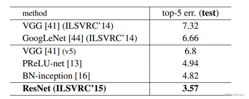
On the ImageNet dataset, the author used a 152-layer ResNet, which is 8 times deeper than VGG19, but still has fewer parameters. An ensemble of these ResNets produced an error rate of only 3.7% on the ImageNet test set, a result that won the ILSVRC 2015 competition. On the COCO object detection dataset, it also yields a 28% relative improvement due to its deep representation.

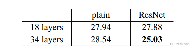
• The above results show that the shortcut connection will be able to solve the problem caused by increasing the number of layers, because when we increase the number of layers from 18 to 34, the error rate on the ImageNet validation set will also decrease unlike ordinary networks.
  
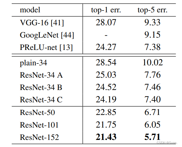
• Below are the results on the ImageNet test set. The top 5 error rate of ResNet is 3.57%, which is the lowest, so the ResNet architecture ranked first in the 2015 ImageNet classification challenge.