Table of contents
2.1 Why propose the residual structure
3.1 ResNet structure with different configurations
3.2 Comparison of Residual Structure Effects
3.3 In the residual structure, how to deal with inconsistent input and output dimensions
3.4 Deep ResNet introduces the bottleneck structure Botleneck
Paper address: https://arxiv.org/pdf/1512.03385.pdf
Video: ResNet that supports half the sky of computer vision [Paper Intensive Reading]_哔哩哔哩_bilibili
Code: 7.6. Residual Networks (ResNet) — Hands-on Deep Learning 2.0.0 documentation
1 summary
main content
Deep neural networks are difficult to train, and we use residual (residual structure) to make network training much easier than before. The 152-layer ResNet was used on ImageNet, which is 8 times more than VGG, but the computational complexity is lower, and finally won the first place in the classification task of ImageNet2015. Train a network of 100-1000 layers on cifar-10. Just by replacing the previous network with a residual network, a 28% improvement was obtained on the coco dataset. Also won the first place in ImageNet target detection, coco target detection and coco segmentation.
main chart
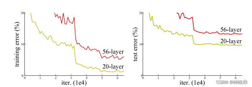
The above picture shows the network training error and test error without using the residual structure. The results show that the training error and test error of the deeper layer are higher than those of the shallow layer, that is, the deep network is actually not trained. The picture below is a comparison of network effects using the resnet structure. It can be seen that after using the residual structure on the right, the 34-layer network training and testing errors are lower.

2 Introduction
2.1 Why propose the residual structure
Deep convolutional neural networks are very effective because many layers can be stacked, and different layers can represent features of different levels. However, it is difficult to optimize when the network is very deep, because gradient disappearance or gradient explosion is prone to occur. The solution is to initialize a good network weight so that the weight cannot be too large or too small; the second is to add some normalization, such as BN, so that The output between each layer, as well as the mean and variance of the gradient can be checked to avoid some layers being too large or too small, so that a deeper network can be trained (can converge). But there is another problem, the performance of the deep network will be worse, and the accuracy will be worse.
The poor performance of the deep network is not due to overfitting due to the large number of network layers and the complexity of the model, because overfitting means that the training error is low and the test error is high, and the training error here also becomes high. So why is this happening? Theoretically speaking, if you add some layers to a shallow network to get a deeper network, the accuracy of the latter should not be worse at least, because the latter at least allows the newly added layer to do identity mapping, while other layers directly copied from the former . If the newly added layers can be trained to at least identity mapping, then the new model will be as effective as the original model. At the same time, because the new model is more complex, it is possible to obtain a better solution to fit the training data set and reduce the training error. But in fact, the SGD optimizer cannot find this better solution.
Therefore, the author explicitly constructs an identity mapping. If the learning effect of some layers is not good, then at least do the identity mapping, so as not to affect the learning of the later layers, so that the accuracy of the deep model will at least not become worse. Assume that after adding some new layers to the original layer, the mapping to be learned is H(x), but the new layer does not learn H(x) directly, but learns H(x)−x, this part uses F( x) means. That is, the newly added layer learns the residual function F(x) = H(x) - x. The final output of the model is F(x)+x. This newly added layer is residual. The goal of optimization becomes F(x).
The structure is shown in the figure below (right):
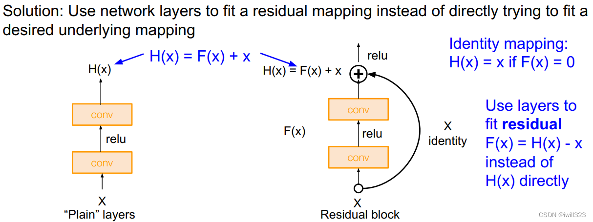
F(x)+x is a direct addition in mathematics, and it is realized through shortcut connections in the neural network (shortcut is to skip one or more layers and directly add the input to the output of these skipped layers). The shortcut actually does an identity mapping (identity mapping), and this operation does not need to learn any parameters, and does not increase the complexity of the model. There is only one more addition, and the amount of calculation is not increased. The network structure is basically unchanged and can be trained normally.
2.2 Experimental verification
A series of experiments were done on imagenet for verification. The results show that 1) the residual network is easy to optimize, and 2) the accuracy of the residual network will increase due to the deeper network stack.
3 Experimental part
3.1 ResNet structure with different configurations

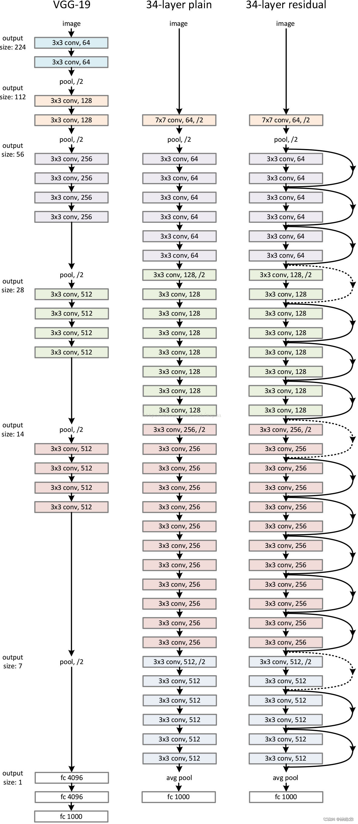
Compare the ResNet34 structure diagram below: (3+4+6+3)=16 residual modules, each with two convolutional layers. Plus the first 7×7 convolutional layer and the last fully connected layer, a total of 34 layers.
3.2 Comparison of Residual Structure Effects

three major observations:
- 34 layers is better than 18 layers, the degradation problem is solved
- Faster convergence and better convergence results using residuals
- 对于18层,The 18-layer plain/residual nets are comparably accurate, but the 18-layer ResNet converges faster
3.3 In the residual structure, how to deal with inconsistent input and output dimensions
A. The pad is filled with 0 to make the dimensions consistent;
B. When the dimensions are inconsistent, make it mapped to a unified dimension, such as using full connection or 1×1 convolution in CNN, so that the output channel is twice the input. In resnet, if the number of output channels is doubled, the height and width of the input are usually halved, so 1×1 convolution stride=2
C. Projection mapping is performed regardless of whether the input and output dimensions are consistent.
The following authors verify the effects of these three operations. As can be seen from the results below, B and C have similar effects, and both are better than A. However, mapping will add a lot of complexity. Considering that the input and output dimensions are the same in most cases in ResNet (the number of channels will change when only 4 modules are connected ), the author finally adopted plan B.

3.4 Deep ResNet introduces the bottleneck structure Botleneck
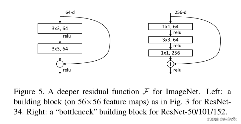
In the structure of ResNet-50 and above, the model is deeper and more patterns can be learned, so the number of channels must also increase. For example, in the previous model configuration table, the output of the first residual module of ResNet-50/101/152 is 256 dimensions, compared with 64 dimensions, it is increased to 4 times, and the calculation amount is increased to 16 times, which is not worthwhile.
The Bottleneck structure is designed to improve efficiency. For example, for the first module, after a 1×1 convolution, the input is reduced from 256 dimensions to 64 dimensions, then a 3×3 convolution is performed, and the dimension is increased back to 256 dimensions after a 1×1 convolution. After doing this, the complexity is about the same as that shown on the left. Therefore, the theoretical calculation amount of ResNet-50 compared with ResNet-34 has not changed much. But in fact, the calculation efficiency of 1×1 convolution is not as high as that of other convolutions, so the calculation of ResNet-50 is still more expensive.
4 code implementation
4.1 Residual block
ResNet follows VGG's complete 3×3 convolutional layer design.
- In the residual block, there are first two 3×3 convolutional layers with the same number of output channels, and each convolutional layer is followed by a batch normalization layer and a ReLU activation function.
- If the output of the two convolutional layers has the same shape as the input, the input is directly added to the final ReLU activation function through the cross-layer data path.
- If you want to change the number of channels, you need to introduce an additional 1×1 convolutional layer to transform the input into the required shape, and then do the addition operation.
class Residual(nn.Module):
    def __init__(self, input_channels, num_channels, use_1x1conv=False, strides=1):
        super().__init__()
        self.conv1 = nn.Conv2d(input_channels, num_channels,
                               kernel_size=3, padding=1, stride=strides)
        self.conv2 = nn.Conv2d(num_channels, num_channels,
                               kernel_size=3, padding=1)
        if use_1x1conv:
            self.conv3 = nn.Conv2d(input_channels, num_channels,
                                   kernel_size=1, stride=strides)
        else:
            self.conv3 = None
        self.bn1 = nn.BatchNorm2d(num_channels)
        self.bn2 = nn.BatchNorm2d(num_channels)


    def forward(self, X):
        Y = F.relu(self.bn1(self.conv1(X)))
        Y = self.bn2(self.conv2(Y))
        if self.conv3:
            X = self.conv3(X)
        Y += X
        return F.relu(Y)
This code generates two kinds of residual blocks: (use_1x1conv=True/False)
- The stride is 2, the height and width are halved, and the number of channels is increased. So the shortcut connection part will add a 1×1 convolutional layer to change the number of channels
blk = Residual(3,6, use_1x1conv=True, strides=2)
blk(X).shapetorch.Size([4, 6, 3, 3])
- With a stride of 1 and constant height and width, the input is added to the output (before applying the ReLU nonlinearity)
blk = Residual(3,3)
X = torch.rand(4, 3, 6, 6)
Y = blk(X)
Y.shapetorch.Size([4, 3, 6, 6])

The above implementation is a bit different from pytorch. When pytorch was implemented, bath norm was also done after use_1x1conv:
if stride != 1 or self.inplanes != planes * block.expansion:
            downsample = nn.Sequential(
                conv1x1(self.inplanes, planes * block.expansion, stride),
                norm_layer(planes * block.expansion),
            )
The 1X1 convolution used:
def conv1x1(in_planes: int, out_planes: int, stride: int = 1) -> nn.Conv2d:
    """1x1 convolution"""
    return nn.Conv2d(in_planes, out_planes, kernel_size=1, stride=stride, bias=False)
4.2 ResNet model
Full ResNet architecture:
- Stack residual blocks
- Every residual block has two 3x3 conv layers
- Periodically, double of filters and downsample spatially using stride 2 (/2 in each dimension)
- Additional conv layer at the beginning (stem)
- No FC layers at the end (only FC 1000 to output classes)
- In theory, you can train a ResNet with input image of variable sizes
- Global average pooling layer after last conv layer
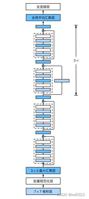
The first two layers of ResNet are the same as those in GoogLeNet: after the 7×7 convolutional layer with 64 output channels and a stride of 2, it is followed by a 3×3 maximum pooling layer with a stride of 2. The difference is that ResNet adds a batch normalization layer after each convolutional layer.
b1 = nn.Sequential(nn.Conv2d(1, 64, kernel_size=7, stride=2, padding=3),
                   nn.BatchNorm2d(64), nn.ReLU(),
                   nn.MaxPool2d(kernel_size=3, stride=2, padding=1))
Below, ResNet uses 4 modules composed of residual blocks, and each module uses several residual blocks with the same number of output channels.
- For the first module: the number of output channels is the same as the number of input channels, so there is no need to use 1x1conv; since the maximum pooling layer with a stride of 2 has been used before, there is no need to reduce the height and width.
- For each subsequent module: In the first residual block, the number of output channels is inconsistent with the number of input channels, so 1x1conv is used; the first residual block doubles the number of channels of the previous module, and the height and width cut in half.
def resnet_block(input_channels, num_channels, num_residuals,
                 first_block=False):
    blk = []
    for i in range(num_residuals):
        if i == 0 and not first_block:
            blk.append(Residual(input_channels, num_channels,
                                use_1x1conv=True, strides=2))
        else:
            blk.append(Residual(num_channels, num_channels))
    return blk

b2 = nn.Sequential(*resnet_block(64, 64, 2, first_block=True))
b3 = nn.Sequential(*resnet_block(64, 128, 2))
b4 = nn.Sequential(*resnet_block(128, 256, 2))
b5 = nn.Sequential(*resnet_block(256, 512, 2))
Global average pooling layer, and fully connected layer output
net = nn.Sequential(b1, b2, b3, b4, b5,
                    nn.AdaptiveAvgPool2d((1,1)),
                    nn.Flatten(), nn.Linear(512, 10))
Observe how the input shape of different modules in ResNet changes
X = torch.rand(size=(1, 1, 224, 224))
for layer in net:
    X = layer(X)
    print(layer.__class__.__name__,'output shape:\t', X.shape)
Sequential output shape: torch.Size([1, 64, 56, 56])
Sequential output shape: torch.Size([1, 128, 28, 28])
Sequential output shape: torch.Size([1, 256, 14, 14])
Sequential output shape: torch.Size([1, 512, 7, 7])
AdaptiveAvgPool2d output shape: torch.Size([1, 512, 1, 1])
Flatten output shape: torch.Size([1, 512])
Linear output shape: torch.Size([1, 10])
Each module has 4 convolutional layers (not including the 1×1 convolutional layer for the identity map). Adding the first 7×7 convolutional layer and the last fully connected layer, there are 18 layers in total. Therefore, this model is often called ResNet-18. Different ResNet models can be obtained by configuring different numbers of channels and residual blocks in the module, such as a deeper ResNet-152 with 152 layers. Although the main architecture of ResNet is similar to GoogLeNet, the ResNet architecture is simpler and more convenient to modify. These factors have led to the rapid and widespread use of ResNet
Full code:
class Residual_Block(nn.Module):
    def __init__(self, ic, oc, stride=1):
        super().__init__()
        self.conv1 = nn.Sequential(
            nn.Conv2d(ic, oc, kernel_size=3, padding=1, stride=stride),
            nn.BatchNorm2d(oc),
            nn.ReLU(inplace=True)
        )

        self.conv2 = nn.Sequential(
            nn.Conv2d(oc, oc, kernel_size=3, padding=1),
            nn.BatchNorm2d(oc)
        )

        self.relu = nn.ReLU(inplace=True)

        if stride != 1 or (ic != oc):  # 对于resnet18,or的两个条件一直,因为改变通道的时候,同时stride == 2
            self.conv3 = nn.Sequential(
                nn.Conv2d(ic, oc, kernel_size=1, stride=stride),
                nn.BatchNorm2d(oc)
            )
        else:
            self.conv3 = None

    def forward(self, X):
        Y = self.conv1(X)
        Y = self.conv2(Y)
        if self.conv3:
            X = self.conv3(X)
        Y += X
        return self.relu(Y)


class ResNet(nn.Module):
    def __init__(self, block = Residual_Block, num_layers = [2,2,2,2], num_classes=11):
        super().__init__()
        self.preconv = nn.Sequential(
            nn.Conv2d(3, 64, kernel_size=7, stride=2, padding=3),
            nn.BatchNorm2d(64),
            nn.ReLU(),
            nn.MaxPool2d(kernel_size=3, stride=2, padding=1)
        )

        self.layer0 = self.make_residual(block, 64, 64,  num_layers[0])
        self.layer1 = self.make_residual(block, 64, 128, num_layers[1], stride=2)
        self.layer2 = self.make_residual(block, 128, 256, num_layers[2], stride=2)
        self.layer3 = self.make_residual(block, 256, 512, num_layers[3], stride=2)

        self.postliner = nn.Sequential(
                    nn.AdaptiveAvgPool2d((1,1)),
                    nn.Flatten(),
                    nn.Linear(512, num_classes)
        )

    def make_residual(self, block, ic, oc, num_layer, stride=1):
        layers = []
        layers.append(block(ic, oc, stride))
        for i in range(1, num_layer):
            layers.append(block(oc, oc))
        return nn.Sequential(*layers)

    def forward(self, x):
        out = self.preconv(x)
        out = self.layer0(out) # [64, 32, 32]
        out = self.layer1(out) # [128, 16, 16]
        out = self.layer2(out) # [256, 8, 8]
        out = self.layer3(out) # [512, 4, 4]
        out = self.postliner(out)
        return out
5 Training and testing
training method
- Image Processing:
- The image is resized with its shorter side randomly sampled in [256, 480].
- A 224×224 crop is randomly sampled from an image or its horizontal flip, with the per-pixel mean subtracted.
- The standard color augmentation is used.
- Batch Normalization after every CONV layer and before activation
- Xavier initialization from He et al.
- SGD + Momentum (0.9) + Weight decay of 1e-5
- Learning rate: starts from 0.1, divided by 10 when validation error plateaus
Manual adjustment is not needed now. Teacher Li believes that even if the change in accuracy has leveled off, it should not jump too early, otherwise the convergence will be weak in the later stage. On the surface, it doesn’t seem to be doing anything, but the model is fine-tuning, but it can’t be seen from the macro data. It’s a good choice to train for a while
- Mini-batch size 256
- No dropout used
test
the standard 10-crop testing: Given a test picture, sample 10 pictures randomly or according to certain rules, make predictions on each sub-picture, and evaluate the results. And not on one resolution, but samples {224, 256, 384, 480, 640} on different resolutions.
6 CIFAR-10 experiments
Why training a 1202-layer network on a small data set like cifar-10 (5w pictures of 32*32), the overfitting is not very powerful. Why the hundreds of billions of parameters of transformer models will not overfit? Li Mu thinks that after adding the residual connection, the intrinsic complexity of the model is greatly reduced. In theory, if some layers are added to the model, the model can at least learn the following layers into identity maps, so that the accuracy will not deteriorate, that is, it is easier to train a simple model to fit the data, so adding a residual connection is equal to the model reduced complexity
7 Why Residual Networks Work
ResNet adds a residual connection to the CNN backbone, so that if the training effect of the newly added layer is not good, at least it can fall back to a simple model, so the accuracy will not deteriorate.
The authors conjecture that fitting the residuals f(x) = H(x) - x is easier. When the ideal mapping f(x) is very close to the identity mapping, the residual mapping is easy to capture the subtle fluctuations of the identity mapping. In fact, it depends on whether this layer has a large change compared with the previous layers, which is equivalent to the role of a differential amplifier.
We hypothesize that it is easier to optimize the residual mapping than to optimize the original, unreferenced mapping
If the optimal function is closer to an identity mapping than to a zero mapping, it should be easier for the solver to find the perturbations with reference to an identity mapping, than to learn the function as a new one.
Looking at it now, ResNet training is faster because the gradient is better maintained . Below g(x) is the original layer, and f() is the newly added layer. A multiplier is added, which causes the newly added layer to easily cause the gradient to disappear, because the gradient is generally small (0-1 Gaussian distribution). The residual connection is added, and the gradient includes the gradient of the previous layer (the item on the right side of the blue plus sign), so that no matter how deep it is added, the gradient will remain relatively large, and the training result will not "lay flat" too quickly (train does not Movement), the more SGD runs, the better the training. The essence of SGD is that as long as the gradient is relatively large, you can keep training. Anyway, there is noise, and it will always converge slowly, and the final effect will be better stochastic gradient descent to optimize life - Zhihu . And because the gradient includes the previously learned item, the residual network learns quickly

Paper recommendation
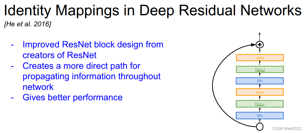
1、Identity Mappings in Deep Residual Networks
A lot of ResidualBlock designs are given in the paper. You can try to achieve several effects by yourself.

2、 Desely Connected Convolutional Networks
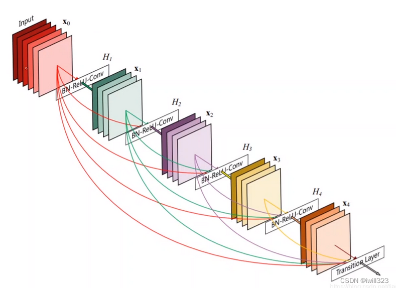
This is also an implementation method worth exploring.