Dahua Deep Residual Network (DRN) ResNet Network Principle

——The original text was published on my WeChat public account "Big Data and Artificial Intelligence Lab" (BigdataAILab). Welcome to pay attention.

When it comes to "deep learning", it is natural to think of its very distinctive features of " deep, deep, deep " (important things are said three times), through a very deep network to achieve very high accuracy image recognition, speech recognition equal ability. Therefore, it is easy to think that a deep network is generally better than a shallow network. If we want to further improve the accuracy of the model, the most direct way is to design the network as deep as possible, so that the accuracy of the model will be improved. will become more and more accurate.

Is that the reality?
Let’s first look at a few classic deep learning models for image recognition:

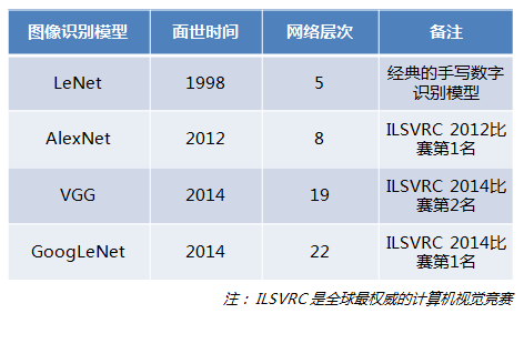
these models are all famous models that have won awards in the world’s top competitions. However, looking at the number of network layers of these models, it seems very disappointing, at least 5 layers, There are only 22 layers. The network level of these world-class models is not that deep. Is this also deep learning? Why not add network layers to hundreds or thousands of layers?

With this question in mind, let's first look at an experiment, stacking many layers directly on the conventional network (plain network, also known as the plain network). After checking the image recognition results, the error results of the training set and test set are as follows:

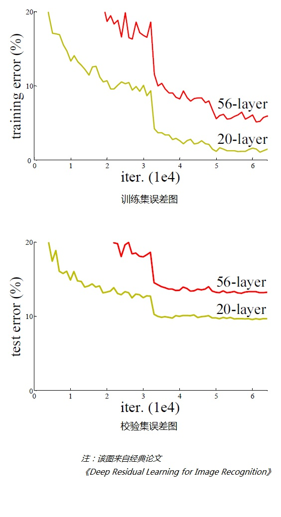
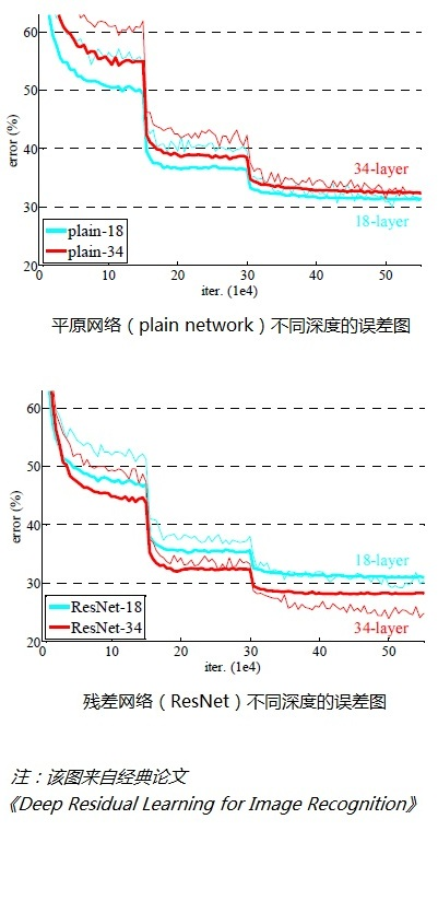
From As can be seen from the above two figures, when the network is very deep (56 layers compared to 20 layers), the model effect is getting worse (the higher the error rate), not the deeper the network, the better.
Through experiments, it can be found that with the continuous increase of the network level, the model accuracy is continuously improved, and when the network level increases to a certain number, the training accuracy and test accuracy decrease rapidly, which shows that when the network becomes very deep, the deep network becomes more difficult to train.

[The question is coming] Why does the model effect deteriorate as the network level gets deeper?

The following figure is a simple neural network diagram, consisting of an input layer, a hidden layer, and an output layer:

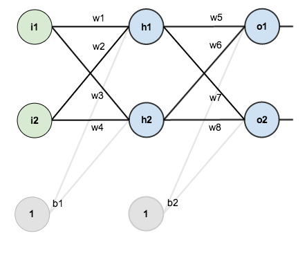
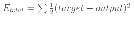
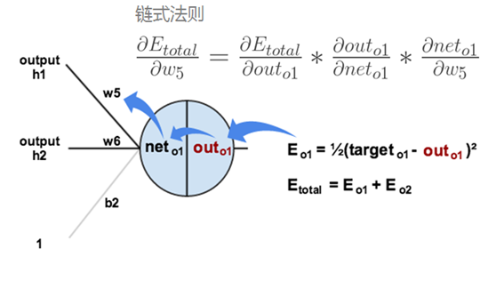
Recall the principle of neural network backpropagation, first calculate the result output through forward propagation, and then compare it with the sample to get the error value Etotal

According to the error results, the famous " chain rule " is used to obtain partial derivatives, so that the resulting error is back-propagated to obtain the gradient of the weight w adjustment. The following figure shows the back-propagation process from the output result to the hidden layer (the back-propagation process from the hidden layer to the input layer is similar):

through continuous iteration, the parameter matrix is continuously adjusted to make the error value of the output result smaller , so that the output is closer to the truth.

It can be seen from the above process that the neural network must continuously propagate the gradient during the backpropagation process, and when the number of network layers deepens, the gradient will gradually disappear during the propagation process (if the Sigmoid function is used, for a signal with an amplitude of 1 , each time a layer is passed backwards, the gradient decays to the original 0.25, the more layers, the more severe the decay), resulting in the inability to effectively adjust the weights of the previous network layers.

So, how to deepen the number of network layers, solve the problem of gradient disappearance, and improve the accuracy of the model?

[Protagonist debut] Deep Residual Network (DRN)

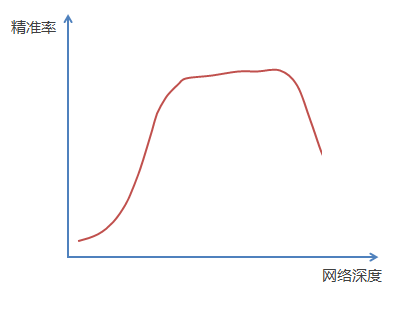
An experimental result phenomenon is described above. When the depth of the neural network is continuously increased, the accuracy of the model will first increase and then reach saturation. When the depth is continuously increased, the accuracy will decrease. The schematic diagram is as follows:

Then we make such an assumption: Suppose A relatively shallow network (Shallow Net) has reached the saturation accuracy rate. At this time, several identity mapping layers (Identity mapping, that is, y=x, the output is equal to the input) are added behind it, so that The depth of the network is increased, and at least the error will not increase, that is, a deeper network should not bring about an increase in the error on the training set. The idea of using identity mapping to directly transfer the output of the previous layer to the back mentioned here is the source of inspiration for the famous deep residual network ResNet.

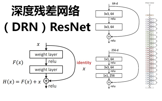
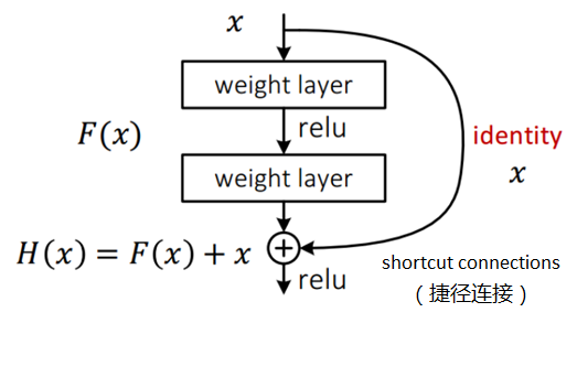
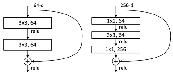
ResNet introduces a residual network structure. Through this residual network structure, the network layer can be made very deep (it is said that it can reach more than 1000 layers at present), and the final classification effect is also very good. The residual network The basic structure is shown in the figure below. Obviously, the figure has a jump structure: the

residual network draws on the idea of cross-layer linking of the Highway Network , but improves it (the residual item is originally a weighted value, but ResNet replaces it with an identity map).
Assuming that the input of a certain neural network is x, and the expected output is H(x), that is, H(x) is the expected complex latent mapping. If you want to learn such a model, the training difficulty will be relatively large;
recall the previous assumptions, If a saturated accuracy rate has been learned (or when it is found that the error of the lower layer becomes larger), then the next learning goal is changed to the learning of the identity mapping, that is, the input x is approximated to the output H(x), so that Staying in the later layers will not cause a loss of accuracy.
In the residual network structure diagram above, the input x is directly passed to the output as the initial result by means of "shortcut connections" , and the output result is H(x)=F(x)+x, when When F(x)=0, then H(x)=x, which is the identity mapping mentioned above. Therefore, ResNet is equivalent to changing the learning target, no longer learning a complete output, but the difference between the target value H(X) and x, which is the so-called residual F(x) := H(x) -x , therefore, the later training goal is to approximate the residual result to 0, so that the accuracy does not decrease as the network deepens.
This residual skipping structure breaks the convention that the output of the n-1 layer of the traditional neural network can only be used as input to the n-layer, so that the output of a certain layer can directly cross several layers as the input of a later layer. , its significance is to provide a new direction for the problem of stacking multi-layer networks so that the error rate of the entire learning model does not drop but rises.
So far, the number of layers of the neural network can exceed the previous constraints, reaching dozens, hundreds or even thousands of layers, which provides feasibility for advanced semantic feature extraction and classification.

Let's feel the structure diagram of the 34-layer deep residual network. Isn't it very spectacular:

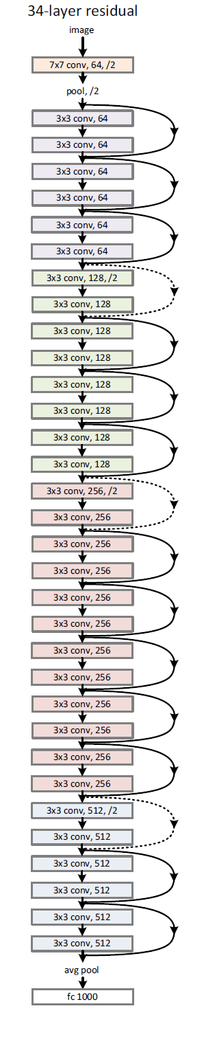
from the figure, we can see how some "shortcut connections" are solid lines and some are dotted lines. What is the difference?

Because after "shortcut connections", H(x)=F(x)+x, if the channels of F(x) and x are the same, they can be added directly, then how to add different channels. The solid line and dotted line in the above figure are to distinguish these two situations:

The Connection part of the solid line indicates that the channels are the same. As shown in the above figure, the first pink rectangle and the third pink rectangle are both 3x3x64 feature maps. Since the channels are the same, the calculation method is H(x)=F(x) +x
The Connection part of the dotted line indicates that the channels are different. As shown in the first green rectangle and the third green rectangle in the above figure, they are the feature maps of 3x3x64 and 3x3x128, respectively. The channels are different, and the calculation method used is H(x)=F(x )+Wx, where W is the convolution operation used to adjust the x dimension.

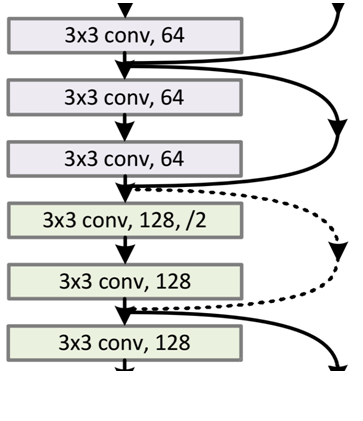
In addition to the two-layer residual learning unit mentioned above, there are also three-layer residual learning units, as shown in the following figure:

the two structures are respectively for ResNet34 (left) and ResNet50/101/152 (right), their main purpose is Just to reduce the number of parameters. The left picture is two 3x3x256 convolutions, the number of parameters: 3x3x256x256x2 = 1179648, the right picture is the first 1x1 convolution to reduce the 256-dimensional channel to 64 dimensions, and then restore it through 1x1 convolution at the end, the overall parameters used Number: 1x1x256x64 + 3x3x64x64 + 1x1x64x256 = 69632, the number of parameters in the right picture is 16.94 times less than that in the left picture. Therefore, the main purpose of the right picture is to reduce the amount of parameters, thereby reducing the amount of calculation.
For regular ResNet, it can be used in networks with 34 layers or less (left image); for deeper networks (such as 101 layers), the right image is used, the purpose of which is to reduce the amount of computation and parameters.

After inspection, the deep residual network does solve the degradation problem. As shown in the figure below, the left picture shows the plain network. The deeper the network layer (34 layers), the higher the error rate than the shallower network layer (18 layers); The picture on the right shows that the deeper the network layer (34 layers) of the residual network ResNet has a lower error rate than the shallower network layer (18 layers).

Conclusion
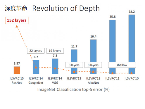
ResNet made a stunning appearance in the ILSVRC2015 competition. It suddenly increased the network depth to 152 layers and reduced the error rate to 3.57. In terms of image recognition error rate and network depth, it has been greatly improved compared to previous competitions. ResNet has no suspense. won the first place in ILSVRC2015. As shown below:

In the second related paper "Identity Mappings in Deep Residual Networks" by the authors of ResNet, ResNet V2 is proposed . The main difference between ResNet V2 and ResNet V1 is that the author found that the feedforward and feedback signals can be directly transmitted by studying the propagation formula of the ResNet residual learning unit, so the nonlinear activation function of "shortcut connection" (such as ReLU) Replaced with Identity Mappings. At the same time, ResNet V2 uses Batch Normalization in each layer. After doing so, the new residual learning unit is easier to train and more generalizable than before.

Wall Crack Advice

It is recommended to carefully read He Kaiming's two classic papers on deep residual networks. The main idea of deep residual networks is proposed in this paper, which is worth collecting and reading.

"Deep Residual Learning for Image Recognition" (image recognition based on deep residual learning)
Identity Mappings in Deep Residual Networks

Scan the following QR code to follow my official account "Big Data and Artificial Intelligence Lab" (BigdataAILab), and then reply to the keyword " thesis " to read the contents of these two classic papers online.

Recommended related reading

Dahua Deep Residual Network (DRN) ResNet Network Principle

Guess you like