Pytorch migrates and trains its own data set

1. Pytorch basic training

The previous section was about basic
video and AI, and interacting with the process (2) pytorch minimally trained its own dataset and recognized it.
Following the previous section, we started to use transfer learning to train our own dataset and save the network, load the network and recognize it.

2. pytorch loads resnet18

The basis of the RetNet network is the residual network, and its original architecture is ResNet. As the name suggests, the depth of the network is 18 layers. Including pooling, activation, linear, excluding batch normalization, pooling, why load resnet18? Because you can use the established model and fine-tune the output, in pytorch, you can use the image classification model pre-trained on ImageNet provided by torchvision to train the deep learning model on the image dataset collected by yourself. This can save a lot of time, using the fine-tuning model, the final resnet18 model output layer is reset, and transfer learning is achieved.

2.1 Standardization of data standardization processing

Definition: Data standardization processing: transforms.Normalize()
Data standardization, generally speaking, the mean (mean) is 0, the standard deviation (std) is 1
Simply put, the data is calculated by channel, and the data of each channel First calculate its variance and mean value, then subtract the mean value from each data in each channel, and then divide it by the variance to get the normalized result. After normalization, the data can better respond to the activation function, improve the expressiveness of the data, and reduce the occurrence of gradient explosion and gradient disappearance.

from __future__ import print_function, division

import torch
import torch.nn as nn
import torch.optim as optim
from torch.optim import lr_scheduler
import torch.backends.cudnn as cudnn
import numpy as np
import torchvision
from torchvision import datasets, models, transforms
import matplotlib.pyplot as plt
import time
import os
import copy
#通过设置让内置的cuDNN的auto-tuner自动寻找最适合当前配置的高效算法,来达到优化运行效率的问题
device = torch.device("cuda:0" if torch.cuda.is_available() else "cpu")
print(device)
cudnn.benchmark = True
plt.ion()   # interactive mode 交互模式
#定义三个全局变量
dataloaders=None
dataset_sizes =None
class_names = None

Define the normalization function, the value inside is the normalization value of the resnet network, it is not written casually.

#标准化函数
data_transforms = {
    
    
      'train': transforms.Compose([
         transforms.RandomResizedCrop(224),
         transforms.RandomHorizontalFlip(),
         transforms.ToTensor(),
         transforms.Normalize([0.485, 0.456, 0.406], [0.229, 0.224, 0.225])
       ]),
      'val': transforms.Compose([
         transforms.Resize(256),
         transforms.CenterCrop(224),
         transforms.ToTensor(),

      ]),
   } 

2.2 Training function

Next, write the training function, the parameters have been explained

def train_model(model, criterion, optimizer, scheduler, num_epochs=25): 
    """ 训练模型，并返回在最佳模型 
    参数: 
    - model(nn.Module): 要训练的模型 
    - criterion: 损失函数 
    - optimizer(optim.Optimizer): 优化器 
    - scheduler:                  学习率调度器 
    - num_epochs(int):            最大 epoch 数 
    返回: 
    - model(nn.Module):           最佳模型 
    - best_acc(float):            checkpoint最好准确率 
    """
    since = time.time()
    best_model_wts = copy.deepcopy(model.state_dict())
    best_acc = 0.0

    for epoch in range(num_epochs):
        print(f'Epoch {
      
      epoch}/{
      
      num_epochs - 1}')
        print('-' * 10)

        # 训练集和验证集交替进行前向传播
        for phase in ['train', 'val']:
            if phase == 'train':
                model.train()  # 设置为训练模式，可以更新网络参数
            else:
                model.eval()   # 设置为预估模式，不可更新网络参数

            running_loss = 0.0
            running_corrects = 0

            # 遍历数据集
            for inputs, labels in dataloaders[phase]:
                global device
                inputs = inputs.to(device)
                labels = labels.to(device)

                # 清空梯度，避免累加了上一次的梯度
                optimizer.zero_grad()

                with torch.set_grad_enabled(phase == 'train'):
                    # 正向传播
                    outputs = model(inputs)
                    _, preds = torch.max(outputs, 1)
                    loss = criterion(outputs, labels)

                    # 反向传播且仅在训练阶段进行优化
                    if phase == 'train':
                        loss.backward() # 反向传播
                        optimizer.step()

                # 统计loss、准确率
                running_loss += loss.item() * inputs.size(0)
                running_corrects += torch.sum(preds == labels.data)
            if phase == 'train':
                scheduler.step()

            epoch_loss = running_loss / dataset_sizes[phase]
            epoch_acc = running_corrects.double() / dataset_sizes[phase]

            print(f'{
      
      phase} Loss: {
      
      epoch_loss:.4f} Acc: {
      
      epoch_acc:.4f}')

            # 发现了更优的模型，记录起来
            if phase == 'val' and epoch_acc > best_acc:
                best_acc = epoch_acc
                best_model_wts = copy.deepcopy(model.state_dict())

        print()

    time_elapsed = time.time() - since
    print(f'Training complete in {
      
      time_elapsed // 60:.0f}m {
      
      time_elapsed % 60:.0f}s')
    print(f'Best val Acc: {
      
      best_acc:4f}')

    # 加载训练的最好的模型
    model.load_state_dict(best_model_wts)
    return model

3. Dataset loading and placement

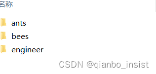
Place two directories under the data directory, one is train, the other is val, which are obviously the training set and the verification set. There are

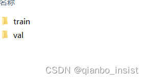
three categories, ants, bees and engineering vehicles. The engineering vehicles use the content in the previous article.

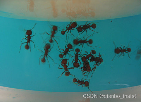
The image of the construction vehicle is as follows, just put it away, and the verification set is the same.
The code list is as follows:

from __future__ import print_function, division

import torch
import torch.nn as nn
import torch.optim as optim
from torch.optim import lr_scheduler
import torch.backends.cudnn as cudnn
import numpy as np
import torchvision
from torchvision import datasets, models, transforms
import matplotlib.pyplot as plt
import time
import os
import copy
#通过设置让内置的cuDNN的auto-tuner自动寻找最适合当前配置的高效算法,来达到优化运行效率的问题
device = torch.device("cuda:0" if torch.cuda.is_available() else "cpu")
print(device)
cudnn.benchmark = True
plt.ion()   # interactive mode 交互模式
dataloaders=None
dataset_sizes =None
class_names = None

def imshow(inp, title=None): 
    # 可视化一组 Tensor 的图片
    inp = inp.numpy().transpose((1, 2, 0)) 
    mean = np.array([0.485, 0.456, 0.406]) 
    std = np.array([0.229, 0.224, 0.225]) 
    inp = std * inp + mean 
    inp = np.clip(inp, 0, 1) 
    plt.imshow(inp) 
    if title is not None: 
        plt.title(title) 
    plt.pause(0.001) # 暂停一会儿，为了将图片显示出来

def train_model(model, criterion, optimizer, scheduler, num_epochs=25): 
    """ 训练模型，并返回在验证集上的最佳模型和准确率 
    Args: 
    - model(nn.Module): 要训练的模型 
    - criterion: 损失函数 
    - optimizer(optim.Optimizer): 优化器 
    - scheduler: 学习率调度器 
    - num_epochs(int): 最大 epoch 数 
    Return: 
    - model(nn.Module): 最佳模型 
    - best_acc(float): 最佳准确率 
    """
    since = time.time()

    best_model_wts = copy.deepcopy(model.state_dict())
    best_acc = 0.0

    for epoch in range(num_epochs):
        print(f'Epoch {
      
      epoch}/{
      
      num_epochs - 1}')
        print('-' * 10)

        # 训练集和验证集交替进行前向传播
        for phase in ['train', 'val']:
            if phase == 'train':
                model.train()  # 设置为训练模式，可以更新网络参数
            else:
                model.eval()   # 设置为预估模式，不可更新网络参数

            running_loss = 0.0
            running_corrects = 0

            # 遍历数据集
            for inputs, labels in dataloaders[phase]:
                global device
                inputs = inputs.to(device)
                labels = labels.to(device)

                # 清空梯度，避免累加了上一次的梯度
                optimizer.zero_grad()

                with torch.set_grad_enabled(phase == 'train'):
                    # 正向传播
                    outputs = model(inputs)
                    _, preds = torch.max(outputs, 1)
                    loss = criterion(outputs, labels)

                    # 反向传播且仅在训练阶段进行优化
                    if phase == 'train':
                        loss.backward() # 反向传播
                        optimizer.step()

                # 统计loss、准确率
                running_loss += loss.item() * inputs.size(0)
                running_corrects += torch.sum(preds == labels.data)
            if phase == 'train':
                scheduler.step()

            epoch_loss = running_loss / dataset_sizes[phase]
            epoch_acc = running_corrects.double() / dataset_sizes[phase]

            print(f'{
      
      phase} Loss: {
      
      epoch_loss:.4f} Acc: {
      
      epoch_acc:.4f}')

            # 发现了更优的模型，记录起来
            if phase == 'val' and epoch_acc > best_acc:
                best_acc = epoch_acc
                best_model_wts = copy.deepcopy(model.state_dict())

        print()

    time_elapsed = time.time() - since
    print(f'Training complete in {
      
      time_elapsed // 60:.0f}m {
      
      time_elapsed % 60:.0f}s')
    print(f'Best val Acc: {
      
      best_acc:4f}')

    # 加载训练的最好的模型
    model.load_state_dict(best_model_wts)
    return model

def visualize_model(model, num_images=6):
    was_training = model.training
    model.eval()
    images_so_far = 0
    fig = plt.figure()

    with torch.no_grad():
        for i, (inputs, labels) in enumerate(dataloaders['val']):
            global device
            inputs = inputs.to(device)
            labels = labels.to(device)
            outputs = model(inputs)
            _, preds = torch.max(outputs, 1)

            for j in range(inputs.size()[0]):
                images_so_far += 1
                ax = plt.subplot(num_images//2, 2, images_so_far)
                ax.axis('off')
                ax.set_title(f'predicted: {
      
      class_names[preds[j]]}')
                imshow(inputs.cpu().data[j])

                if images_so_far == num_images:
                    model.train(mode=was_training)
                    return
        model.train(mode=was_training)

def main():
   # 在训练集上：扩充、归一化
   # 在验证集上：归一化
   data_transforms = {
    
    
      'train': transforms.Compose([
         transforms.RandomResizedCrop(224),
         transforms.RandomHorizontalFlip(),
         transforms.ToTensor(),
         transforms.Normalize([0.485, 0.456, 0.406], [0.229, 0.224, 0.225])
       ]),
      'val': transforms.Compose([
         transforms.Resize(256),
         transforms.CenterCrop(224),
         transforms.ToTensor(),

      ]),
   } 
   data_dir = './data'
   image_datasets = {
    
    x: datasets.ImageFolder(os.path.join(data_dir, x),
                                                data_transforms[x])
                        for x in ['train', 'val']}
   global dataloaders
   dataloaders = {
    
    x: torch.utils.data.DataLoader(image_datasets[x], batch_size=4,
                                                    shuffle=True, num_workers=4)
                    for x in ['train', 'val']}
   global dataset_sizes
   dataset_sizes = {
    
    x: len(image_datasets[x]) for x in ['train', 'val']}
   
   global class_names
   class_names = image_datasets['train'].classes

   print(class_names)

   # 获取一批训练数据
   inputs, classes = next(iter(dataloaders['train'])) 
   # 批量制作网格
   out = torchvision.utils.make_grid(inputs) 
   imshow(out, title=[class_names[x] for x in classes]) 


   model = models.resnet18(pretrained=True) # 加载预训练模型
   for param in model.parameters():
        param.requires_grad = False
   num_ftrs = model.fc.in_features # 获取低级特征维度 
   model.fc = nn.Linear(num_ftrs, 3) # 替换新的输出层 
   model = model.to(device) 
   # 交叉熵作为损失函数 
   criterion = nn.CrossEntropyLoss() 
   # 所有参数都参加训练 
   optimizer_ft = optim.SGD(model.parameters(), lr=0.001, momentum=0.9) 
   # 每过 7 个 epoch 将学习率变为原来的 0.1 
   scheduler = optim.lr_scheduler.StepLR(optimizer_ft, step_size=7, gamma=0.1)
   model_ft = train_model(model, criterion, optimizer_ft, scheduler, num_epochs=3) # 开始训练 
   visualize_model(model_ft)
   PATH = './test.pth'
   torch.save(model_ft.state_dict(), PATH)



if __name__== "__main__" :
  main()

4. How to call

We saved the pth file earlier, but actually used state_dict, which is different from direct model saving

import torch
from PIL import Image
import torchvision.transforms as transforms
import matplotlib.pyplot as plt
import numpy as np
import torch.nn as nn
from torchvision import models
device = torch.device("cuda:0" if torch.cuda.is_available() else "cpu")
PATH = './test.pth'
transform = transforms.Compose(
    [transforms.Resize((256, 256)),transforms.ToTensor(),
     transforms.Normalize((0.485, 0.456, 0.406), (0.229, 0.224, 0.225))])




model = models.resnet18(pretrained=True) # 加载预训练模型
num_ftrs = model.fc.in_features # 获取低级特征维度 
model.fc = nn.Linear(num_ftrs, 3) # 替换新的输出层 
print(device)
model = model.to(device) 
model.load_state_dict(torch.load(PATH))
model.eval()

img = Image.open("./ant.jpg") .convert('RGB')


img = transform(img)
img = img.unsqueeze(0)
img = img.to(device)
with torch.no_grad():
    outputs = model(img)
    _, predicted = torch.max(outputs.data, 1)
    print("the test img lable is ",predicted)

The unsqueeze function inside is necessary. Pay attention to this. When loading an image, the image usually has 3 dimensions, width, height, and number of color channels. For black and white images, the number of color channels is 1, and for color images, there are 3 color channels (red, green and blue, RGB). Therefore, loading an image and storing it as a tensor, the order of dimensions is [channel, height, width], for a two-dimensional convolutional neural network, the three-dimensional data volume cannot correspond. In deep convolutional networks, data is processed in batches. Instead of processing one image at a time, a convolutional neural network processes N images in parallel at the same time. We call this set of images a batch. So instead of dimension [C, H, W], it is [N, C, H, W]. , if you're only processing one image at a time, you still need to put it into a batch form for the model to accept. For example, if you have an image with a shape of [3, 255, 255], you need to convert it to [1, 3, 255, 255]. This is what the unsqueeze(0) function does.

The cuda used during training can be used during recognition, or non-cuda, that is, "cpu", can also be used. The call result is as follows:
python test.py contains ant.jpg

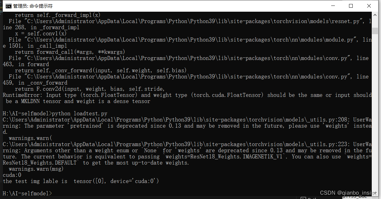
Put an engineering truck in, inside is

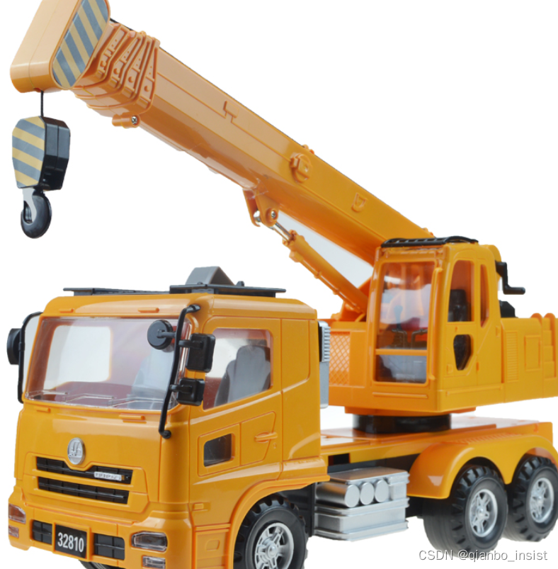
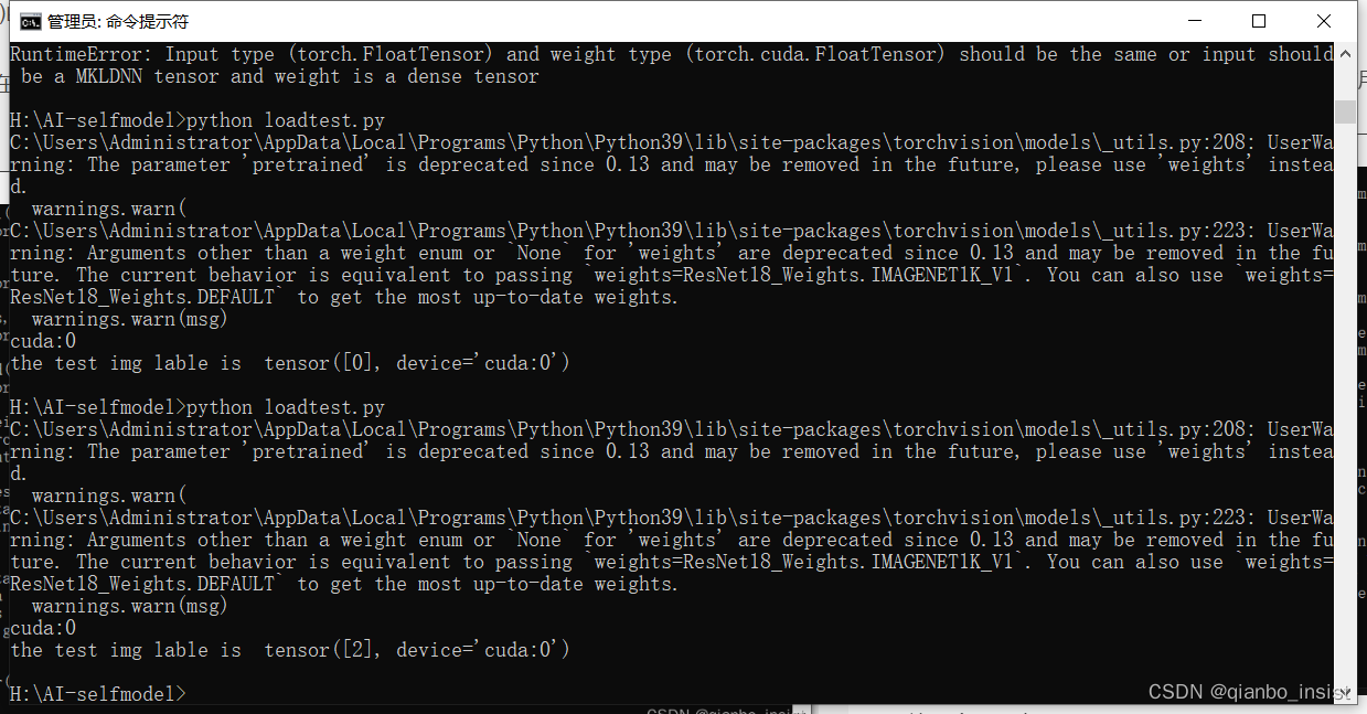
I saw the third category, namely tensor[2], came out, that is, tensor[0] is ant, tensor[1] is bee, tensor[2] is an engineering vehicle

We have completed the training and recognition using migration learning, but there is a limitation here. This is single main object recognition, without multi-classification recognition and target detection. In the next article, we will use multi-classification and target detection to detect objects.