On the overview of efficient fine-tuning of large models: Adapter Tuning, AdaMix, PET, Prefix-Tuning, Prompt Tuning, P-tuning, P-tuning v2

1. Background

  Fine-tuning the pre-trained language model (LM) on downstream tasks has become a paradigm for processing NLP tasks. With the rapid explosion of ChatGPT, it has triggered an era of large-scale models. However, for the general public, pre-training or full fine-tuning of large models is out of reach. As a result, various efficient fine-tuning techniques for parameters have been born, allowing researchers or ordinary developers to have the opportunity to try to fine-tune large models. This article will explain some mainstream fine-tuning techniques.
  The current mainstream large language models are based on the Transformers architecture. Let's briefly introduce Transformers and BERT.

1.1 Dance forms

  Before Transformer, mainstream sequence transformation models were implemented based on complex cyclic or convolutional neural networks, both of which have some disadvantages:

• RNNs: The inherent timing model is difficult to parallelize, and the calculation performance is poor. In addition, there is also the problem of long-distance attenuation
• CNNs: CNN is difficult to model long sequences (because the convolution kernel/receptive field is relatively small during convolution calculation, if the sequence is very long, multi-layer convolution is required to associate two distant positions). But if you use Transformer's attention mechanism, you can see all the positions in the sequence every time (one layer), so there is no such problem.

  Transformer is the first fully attention-based sequential transformation model, multi-headed self-attentionreplacing the most commonly used recurrent layers in encoder-decoderthe architecture . But the advantage of convolution is that the output can have multiple channels, and each channel can be considered to recognize different patterns. The author also wants to obtain the effect of this multi-channel output, so he proposed the Multi-Head Attention multi-head attention mechanism (analog volume multi-channel output effect).

1.1.1 Model structure

The overall architecture of the Transformer is as follows:

Encoder : The encoder consists of N=6 identical encoder layer stacks. Each layer has two sublayers.

1. multi-head self-attention

2. The FFNN layer (Feed Forward Neural Network layer, Feed Forward Neural Network) is actually MLP. For fancy, the name is very long.

   • Both sublayers use residual connections followed by layer normalization.
   • The output of each sublayer is LayerNorm(x + Sublayer(x)), where Sublayer(x) is the output of the current sublayer.
   • For simplicity, all sublayers in the model, as well as the embedding layer, have vector dimensions $d_{\text{model}}=512$ (If the input and output dimensions are different, the residual connection needs to be projected to map it to a unified dimension). (This is different from the previous CNN or MLP approach, and some downsampling will be performed before)

  This unified dimension of each layer makes the model relatively simple, only N and $d_{\text{model}}$Two parameters need to be tuned. This also affects a series of networks behind, such as bert and GPT and so on.

Decoder : The decoder also consists of N=6 stacks of identical decoder layers, each with three sublayers.

1. Masked multi-head self-attention
   In the decoder, the Self Attention layer only allows attention to words in the output sequence that are earlier than the current position. The specific method is: before the Self Attention score passes through the Softmax layer, use the attention mask to block those positions after the current position. So it is called Masked multi-head self Attention. (Use a large negative number -inf corresponding to the masked position, so that the corresponding value after softmax is 0)

2. Encoder-Decoder Attention
   The encoder outputs the final vector, which will be input to the Encoder-Decoder Attention layer of each decoder to help the decoder focus on the appropriate position of the input sequence.

3. FFNN
FFNNThe layer consists of two linear transformations, and there is a ReLU activation function between the two linear transformations. Similar to the encoder, each sublayer uses a residual connection and then performs layer normalization. Expressed in a formula:
   $$FFN(x,W_1,W_2,b_1,b_2)=W_2\left(relu\right(x{W}_1+b_1))+b_2=max(0,x{W}_1+b_1)W_2+b_2$$

Suppose a Transformer is composed of a 2-layer encoder and a two-layer decoder, as shown in the following figure:

1.1.2 Attention mechanism

1. Scaled Dot-Product Attention (Scaled Dot-Product Attention)
   In practice, we simultaneously compute a set of query attention functions and combine them into a matrix $Q.$ _ Key and value also form a matrix$K$ and$V.$ _ The output matrix we compute is:

$$\mathrm{Attention}(Q,K,V)=\mathrm{softmax}(\frac{Q{K}^T}{\sqrt{d_k}})V$$
2. 多头自注意力，计算公式可表示为：
$$\begin{gathered} \mathrm{MultiHead}(Q,K,V)=\mathrm{Concat}(\mathrm{hea}{\mathrm{d}}_1,...,\mathrm{hea}{\mathrm{d}}_{\mathrm{h}})W^O \\ \text{where}\mathrm{hea}{\mathrm{d}}_{\mathrm{i}}=\mathrm{Attention}(Q{W}_i^Q,K{W}_i^K,V{W}_i^V) \end{gathered}$$
  where the mapping is done by the weight matrix:$W_i^Q\in {\mathbb{R}}^{d_{\text{model}}\times d_k}$, $W_i^K\in R^{d_{\text{model}}\times d_k}$, $W_i^V\in {\mathbb{R}}^{d_{\text{model}}\times d_v}$ and $W^O\in R^{h{d}_v\times d_{\text{model}}}$.
  We take $h=8$ parallel attention layers or heads. For each of these heads we use$d_k=d_v=d_{\text{model}}/h=64$ , the total computational cost is similar to a single head attention with all dimensions.

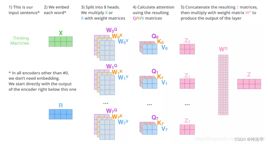
3. Input X and 8 sets of weight matrix$W^Q$, $W^K$ $W^{}$Multiply${}^{V\; to\; get\; 8\; sets\; of\; Q,\; K,\; V\; matrices.}$Carry out attention calculations to get 8 groups of Z matrices (assuming head=8)
4. Concatenate the 8 groups of matrices and multiply them by the weight matrix$W^O$ , map it back to a d-dimensional vector (equivalent to the aggregation of multi-dimensional features), and get the final matrix Z. This matrix contains information about all attention heads.
5. The matrix Z will be input to the FFNN layer. (The feedforward neural network layer also receives 1 matrix instead of 8. The vector of each row represents a word)

1.1.3 Application of Attention in Transformer

Multi-head attention is used in 3 different ways in Transformer:

• multi-head self attention: Standard multi-head self-attention layer, used in the first multi-head self-attention layer of the encoder. All keys, values ​​and queries come from the same place, the output of the previous layer in the encoder. In this case, each position in the encoder can pay attention to all positions in the layer above the encoder.

• masked-self-attention: Used in decoder, each position of the sequence is only allowed to see all positions before the current position. This is to maintain the autoregressive characteristics of the decoder and prevent seeing information about future positions

• encoder-decoder attention: The second multi-head self-attention layer for the encoder block. The query comes from the previous decoder layer, and the keys and values ​​come from the output memory of the encoder, which allows the decoder to focus on the most interesting position in the input sequence at each time step of decoding.

1.2 BERT

  Before BERT came out, the NLP field still constructed its own neural network for each task and then trained it. After BERT comes out, you can pre-train a model to apply it to many different NLP tasks. It simplifies training and improves its performance. BERT and subsequent work have made NLP a qualitative leap in the past few years.

  BERT consists of two parts: pre-training and fine-tuning. In order to handle a variety of tasks, the BERT input can be a sentence or a sentence pair. The entire BERT structure is as follows:

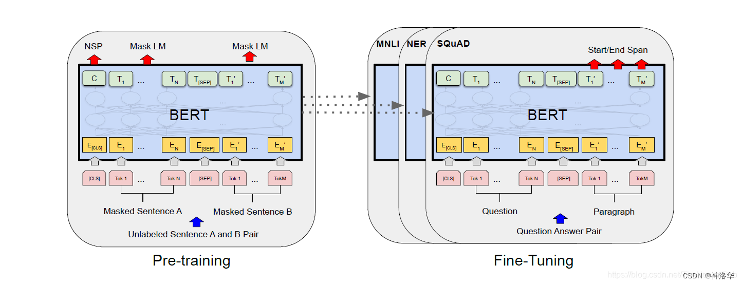
• [CLS]: That is, classification, placed at the beginning of the sentence, represents the information of the entire sequence.
• [SEP]: that is, separate, placed at the end of the sentence, used to separate two sentences
• Use E to represent the input embedding, use $C\in {\mathbb{R}}^H$ to represent the final hidden vector of the special token[CLS], use$T_i\in R^H$ represents the final hidden vector of the i-th input token.

   For each downstream task, we simply concatenate the task-specific inputs and outputs into BERT, and then fine-tune all parameters end-to-end. In the fourth section of the paper, we introduce in detail how to construct input and output according to downstream tasks.

2. PEFTSummary

• 论文《Scaling Down to Scale Up: A Guide to Parameter-Efficient Fine-Tuning》
• huggingface/peft : Integrates LoRA, Prefix Tuning, P-Tuning, Prompt Tuning, AdaLoRA and other PEFT methods
• Refer to Zhihu "Summary of Principles of Efficient Fine-tuning Technology for Large Model Parameters"

  Parameter-efficient fine-tuning ( PEFTParameter-efficient fine-tuning ) aims to solve this problem by training only a small set of parameters, which may be a subset of existing model parameters or a newly added set of parameters. These methods differ in parameter efficiency, memory efficiency, training speed, final quality of the model, and additional inference cost (if any). This paper provides a systematic overview, division, and comparison of 40 papers on efficient fine-tuning methods for models published between February 2019 and February 2023.

2.1 Classification of PEFT

  PEFT methods can be classified in a number of ways, such as by their underlying approach or structure—whether they introduce new parameters to the model, or just fine-tune existing parameters; by fine-tuning purpose—whether they aim to minimize Minimize memory footprint or just pursue storage efficiency. We first classify based on the basic method & structure. The figure below shows the 30 PEFT methods of this classification system.

Figure 2: Classification of parameter efficient fine-tuning methods: Addition-based (Adapter-like methods and Soft prompts), Selection-based, Reparametrization-based.

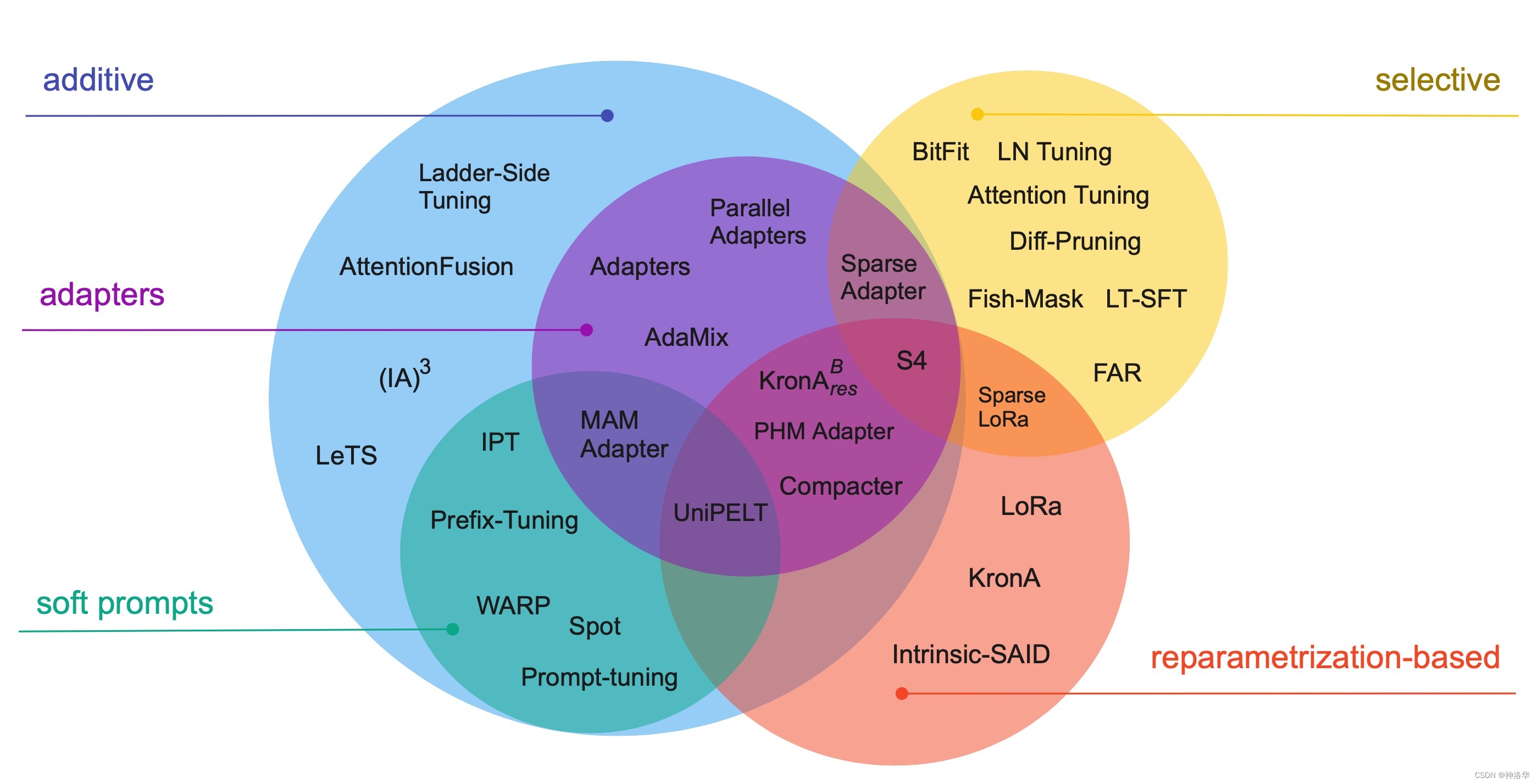
• Additive methods: The main idea is to augment an existing pretrained model by adding additional parameters or layers, and train only the newly added parameters . This is by far the largest and widely explored class of parameter-efficient fine-tuning methods. This method is further divided into:
  • Adapters: That is, a small fully connected network is introduced after the Transformer sublayer, which is widely used. There are several variants of Adapters, such as modifying the position of adapters, pruning, and using reparameterization to reduce the number of trainable parameters.
  • Soft Prompts: GPT-2 aims to control the behavior of language models by modifying the input text. However, these methods are difficult to optimize, and there are limitations such as model input length and the number of training examples, thus introducing the concept of soft. Soft PromptsFine-tuning a portion of the input embeddings of the model via gradient descent transforms the problem of finding hints in a discrete space into a continuous optimization problem. Soft PromptsIt is possible to train only the input layer ( 《GPT Understands, Too》 , Prompt Tuning ), or train all layers ( Prefix-Tuning ).
  • others: e.g. $LeTS$、$LST$ sum$(IA{)}^3$ etc.

  Although these methods introduce additional parameters into the network, they reduce training time and improve memory efficiency by reducing the size of gradients and optimizer states. In addition, the frozen model parameters can be quantized ( refer to the paper ), and additive PEFTthe method can fine-tune larger networks or use larger batch sizes, which improves the training throughput on GPU. Furthermore, optimizing fewer parameters in a distributed setting greatly reduces the amount of communication.

• Selective methods: The earliest selective PEFT method is to fine-tune only a few top layers of the network (freezing the front layer), modern methods are usually based on the type of layer ( Cross-Attention is All You Need ) or internal structure, such as only fine-tuning the bias of the model ( BitFit ) Or just specific lines ( Efficient Fine-Tuning of BERT Models on the Edge ).
• Reparametrization-based PEFT(Reparameterization): Utilizes low-rank representations to minimize the number of trainable parameters. Aghajanyan et al. (2020) demonstrate that fine-tuning can be done efficiently in low-rank subspaces, and for larger models or models pretrained for longer periods of time, smaller subspaces need to be tuned. The most well-known method based on reparameterization is LoRa, which performs a simple low-rank decomposition of the parameter matrix to update the weights $\delta W=W^{down}{W}^{up}$ .${}^{\_}$Recent studies (Karimi Mahabadi et al., 2021; Edalati et al., 2022) also explored Kronecker product reparametrization ($\delta W=A\otimes B$ ), which achieves a more favorable trade-off between rank and number of parameters.
• Hybrid methods: Mix multiple PEFT methods, for example, MAM Adapter combines Adapters and Prompt
  tuning; UniPELT joins LoRa; Compacter and KronAB reparameterize the adapter to reduce its number of parameters; finally, S4 is the result of an automated algorithm search , which combines all PEFT categories, maximizing accuracy with a 0.5% increase in the number of extra parameters.

2.2 Comparison of different PEFT methods

  Parameter efficiency covers multiple aspects, including storage, memory, computation, and performance. However, achieving parameter efficiency alone does not necessarily result in reduced RAM usage.
  To compare PEFT methods, we consider five dimensions: storage efficiency, memory efficiency, computational efficiency, accuracy, and inference overhead, which are not completely independent of each other, but improvements in one dimension do not necessarily lead to improvements in other dimensions.

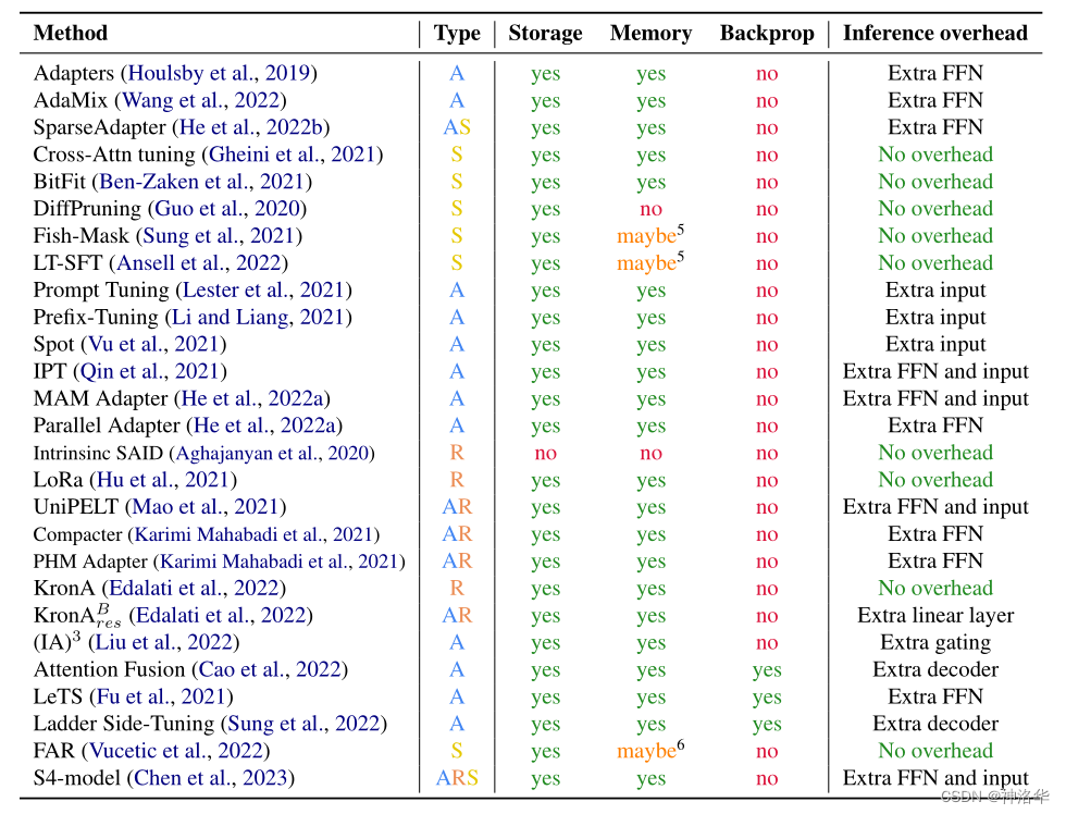
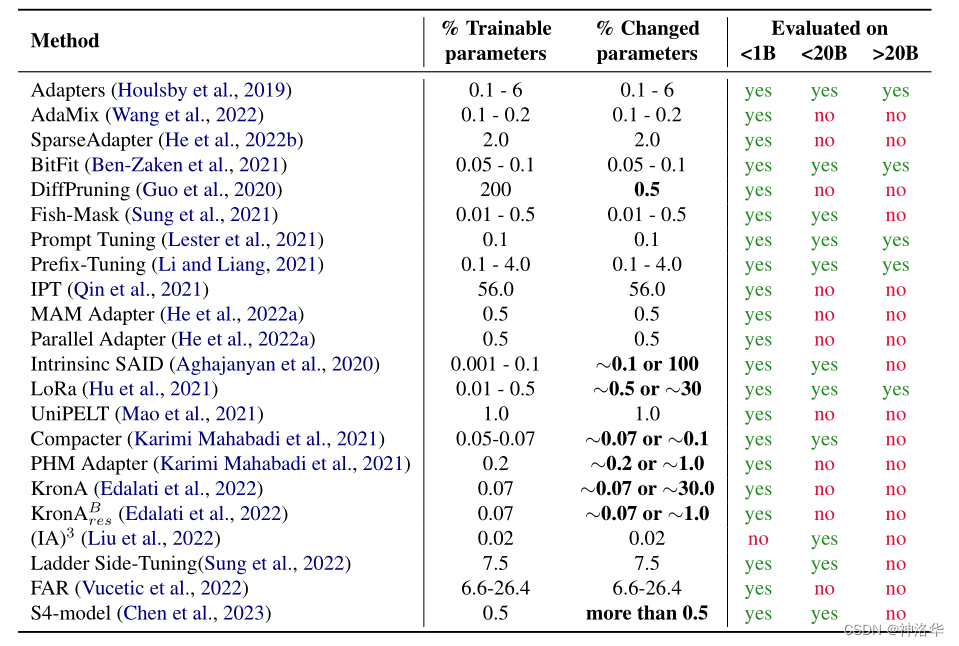
  The following table shows the number of parameters involved in the training (trainable parameters) of various parameter-efficient methods, the amount of changed parameters between the final model and the original model (changed parameters, specifically referring to the number of parameters updated by the gradient optimization algorithm), and the number of parameters involved in the paper. Range of models evaluated (<1B, <20B, >20B)

三、Additive methods

3.1 Adapter Tuning

3.1.1 Adapters（2019.2.2）

Paper "Parameter-Efficient Transfer Learning for NLP"

Adapters originally came from the article "Learning multiple visual domains with residual adapters"   in the CV field . Its core idea is to add some residual modules on the basis of the neural network module, and only optimize these residual modules, because the residual modules have fewer parameters. , so fine-tuning costs are lower .

  Houlsby et al. applied this idea to the field of natural language processing. They propose to add a fully connected network after the Transformer's attention layer and feed-forward neural network (FFN) layer. When fine-tuning, only the newly added Adapter structure and Layer Norm layer are fine-tuned, thus ensuring the efficiency of training. Whenever a new downstream task appears, the Adapter module is added to generate an easily scalable downstream model, thereby avoiding the problems of full fine-tuning and catastrophic forgetting.
  Adapters Tuning is very efficient, and can achieve comparable performance to fine-tuning by fine-tuning less than 4% of the model parameters.

Figure 2. Architecture of the adapter module and its integration with Transformer.

• Left: We add adapter modules twice in each Transformer layer - after multi-head attention post-projection and after two feed-forward layers.
• Right: The adapter as a whole is a bottleneck structure, including two feedforward sublayers (Feedforward) and skip connections (skip-connection).
  • Feedforward down-project: Project the original input dimension d (high-dimensional features) to m (low-dimensional features), and limit the parameter amount of the Adapter module by controlling the size of m. Usually, m<<d;
  • Nonlinearity: nonlinear layer;
  • Feedforward up-project: Restore the input dimension d as the output of the Adapter module. At the same time, the input of the Adapter is added to the final output through a skip connection (residual connection)

def transformer_block_with_adapter(x):
	residual = x
	x = SelfAttention(x)
	x = FFN(x) # adapter
	x = LN(x + residual)
	residual = x
	x = FFN(x) # transformer FFN
	x = FFN(x) # adapter
	x = LN(x + residual)
	return x

  Pfeiffer et al. found that inserting an Adapter after the self-attention layer (after normalization) can achieve performance comparable to the above-mentioned use of two Adapters in the Transformer block.

3.1.2 AdaMix（2022.3.24）

论文《AdaMix: Mixture-of-Adaptations for Parameter-efficient Model Tuning》

3.1.2.1 Mixture-of-Adaptations

In AdaMix, the author defines the Adapter as:

  where out is Feedforward up-projecta mapping ( FFN_Uindicated in this article), and in is Feedforward down-projecta mapping (indicated in this article FFN_D), and the middle nonlinear layer uses the GeLU function. These $E_{i=1}^N$Call it an expert (expert). Inspired by the multi-expert model (MoE: Mixture-of-Experts), this paper proposes Mixture-of-Adapter, which regards each Adapter as an expert.

  In order to sparse the network to keep FLOPs constant, there is an additional gating network $G$ , whose output is a sparse N-dimensional vector. Expert$E$ plus conventional gating unit$G$ , the output of the model can be expressed as:

3.1.2.2 Routing Policy

  Recent work has demonstrated that a stochastic routing policy has the same effect as classical routing mechanisms such as Switch routing, with the following advantages:

• Since input examples are randomly routed to different experts, no additional load balancing is required, as each expert has an equal chance to be activated, simplifying the framework
• The expert-selected Switch layer has no extra parameters and thus no extra calculations, keeping the parameters and FLOPs the same as a single adapter module, which is especially important for our parameter-efficient fine-tuning setup.
• Enable the adapter module to perform different transformations during training and get multiple views of the task

  So for the random routing strategy of the adapter module ( FFN_Uand FFN_Dcan be chosen randomly from different experts), there is: $$x\leftarrow x+f(x\cdot W_{down})\cdot W_{up}$$

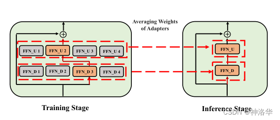
  Taking M = 4 adaptation modules as an example, the AdaMix structure is as follows (including FFN_U, FFN_D and projection matrix):

Figure 2: AdaMix

  As shown in the above figure, firstly, the model only considers one main branch, that is, the left one, to make a loss on the final prediction result; secondly, in order to ensure efficient training, after determining the experts randomly selected by the main branch, the right branch needs to satisfy two FFNs Expert options are all different from the main branch. The loss function is the cross-entropy of the main branch plus the KL consistency loss of the two branches:

  For input $x$ in$On\; L$ Transformer layers. We will specifically add a consistency loss as any regularization term (Consistency regularization), with the aim of making the adapter modules share information and prevent divergence.

  A general summary is to replace the gating unit with a random average selection of experts ( FFN_Uand FFN_Drandom selection), which not only reduces the parameters and calculations consumed by the gating unit, but also ensures that each expert will not be overloaded, and the accuracy is also improved. very good.

3.1.2.3 Pseudocode

def transformer_block_with_adamix(x):
	"""
	实现了带有AdaMix的Transformer块。其中包括自注意力层、残差连接和层归一化、前馈神经网络层以及AdaMix部分的实现
	"""
    residual = x
    x = SelfAttention(x)  # 自注意力层
    x = LN(x + residual)  # 残差连接和层归一化
    residual = x
    x = FFN(x)  # 前馈神经网络层
    # adamix开始
    x = random_choice(experts_up)(x)  # 随机选择上投影的expert
    x = nonlinearity(x)  # 非线性激活函数
    x = random_choice(experts_down)(x)  # 随机选择下投影的expert
    x = LN(x + residual)  # 残差连接和层归一化
    return x

def consistency_regularization(x):
    logits1 = transformer_adamix(x)  # 使用不同的expert计算第一次前向传递的logits
    # 第二次前向传递使用不同的expert
    logits2 = transformer_adamix(x)
    r = symmetrized_KL(logits1, logits2)  # 对称化KL散度作为一致性正则化项
    return r

AdaMix section:

• First, one is randomly selected from the up-projected experts, and the input x is passed to the expert for processing.
• Apply a nonlinear activation function to the output.
• Randomly select one of the down-projected experts, and pass the activated result to the expert for processing.
• Connect the result after the above operations with the residual, then perform layer normalization, and return the result.
  consistency_regularization regardless:
• Use the AdaMix method to make two forward passes on the input x, each time selecting different experts
• Calculate the symmetric KL divergence between the logits obtained by the two forward passes, get the consistency regularization term and return

  The sum in the code experts_upis experts_downthe expert random selection function of the upper projection and the lower projection, symmetrized_KLbut symmetric KL divergence calculation function.

3.1.2.4 Reasoning & Experimental Results

  For the reasoning stage, the article proposes another innovation—mixing all Adapters, that is, violently averaging all Adapter parameters, instead of continuing to use gating units or randomly assigning in the traditional multi-expert model. This is done to make the parameters And the amount of calculation is the smallest and the most efficient.

RoBERTa-largeThe following is the result of using the encoder to perform NLU tasks   on the GLUE development set . It can be seen AdaMixthat it even exceeds the accuracy of fine-tuning the entire model:

the resulting picture is:

3.1.2.5 Summary

  AdaMixMoEAdapter performance is improved by utilizing multiple adapters in a mixture-of-experts manner, which means that each adapter is a set of layers (experts), and only a small set of experts is activated in each forward pass .

  Conventional MoE uses a routing network to select and weight multiple experts, while AdaMix randomly selects an expert in each forward pass, which reduces computational cost without reducing performance. After training, the adapter weights are averaged among experts, which makes inference more efficient.
  To stabilize training, the authors propose consistency regularizationmethods that do this by minimizing the symmetric KL between the forward passes of two different sets of experts selected models. While improving stability, this approach increases computational requirements and memory consumption because it needs to preserve hidden states and gradients in the forward pass of two models with different experts. So, although AdaMix achieves better performance than regular adapters at the same inference cost, it may use more memory during training.

3.1.3 AdapterFusion&AdapterDrop

1. AdapterFusion（EACL 2021 ）

  The advantage of Adapter Tuning is that it only needs to add a small number of new parameters to effectively learn a task, and the parameters of these adapters represent the knowledge required to solve the task to a certain extent. Inspired, the authors ponder whether knowledge from multiple tasks can be combined. To this end, the author proposes AdapterFusiona new two-stage learning algorithm that can utilize knowledge from multiple tasks and outperforms full model fine-tuning and Adapter Tuning in most cases.

2. AdapterDrop（EMNLP 2021 ）

  By analyzing the computational efficiency of the Adapter, the author found that compared with the full fine-tuning, the Adapter is 60% faster in training, but 4%-6% slower in reasoning. Based on this, the author proposes the AdapterDrop method to alleviate this problem. The main methods are:

• Without affecting the performance of the task, the dynamic and efficient removal of the Adapter improves the efficiency of the model in backpropagation (training) and forward propagation (inference). For example, discarding the Adapter in the first five Transformer layers increases the inference speed by 39%, and the performance remains basically the same.
• Prune the Adapter in AdapterFusion. Experiments show that removing most of the Adapters in AdapterFusion to keep only 2 achieves comparable results to the complete AdapterFusion model with eight Adapters, and the inference speed is increased by 68%.

For more details, please refer to "Summary of Principles of Efficient Fine-tuning of Large Model Parameters (4)" .

3.2 Soft Prompts

《Pre-train, Prompt, and Predict: A Systematic Survey of Prompting Methods in Natural Language Processing》

3.2.1 PET（Pattern-Exploiting Training，2020.1）

• 论文《Exploiting Cloze Questions for Few Shot Text Classification and Natural Language Inference》

  The pre-trained language model (such as BERT) contains comprehensive language knowledge and does not target specific downstream tasks. Therefore, when transferring learning directly, the model may not understand exactly what problem you want to solve, what part of knowledge you want to extract, and the final effect Also not good enough.

  After the standard paradigm pre-train, fine-tuneshifts to the new paradigm pre-train, prompt, and predict, instead of adapting language models (LMs) to downstream tasks through target engineering, with the help of text prompts (prompts), the downstream tasks are reformulated to look more like the original LMs trained tasks to be solved during the period. Therefore, the core idea of ​​Prompt is to excavate the specific knowledge in the pre-training model through manual prompts, so as to achieve a good zero-sample effect, and with a small number of labeled samples, the effect can be further improved (improving zero-sample/small- sample learning effect).

  PET uses a template composed of natural language (often called Pattern or Prompt in English) to convert downstream tasks into a cloze task, so that BERT's MLM model can be used for prediction. PETThere are very good zero-sample, small-sample and even semi-supervised learning effects (the training of the MLM model does not require supervised data, so theoretically this can achieve zero-sample learning).

  Of course, this solution is not only feasible for the MLM model. As shown in the figure below, it is actually very simple to use a one-way language model (LM) like GPT. However, since the language model is decoded from left to right, the prediction part can only be placed at the end of the sentence (but the prefix can also be added, but the prediction part is placed at the end).

  However, manual construction of templates is not so easy, and the robustness of discrete text input is very poor, and the effect of different prompt templates is much worse. Finally, such discrete template representations cannot be globally optimized:

  to overcome these difficulties, the concept of soft prompts/continuous prompts is proposed. To put it simply, it is to replace the prompt with a fixed token, splice the text input, and use it as a special embedding input to realize the automatic construction of the template . Transform the discrete optimization problem of finding the best prompt (hard prompt) into a continuous optimization problem, reducing the cost of prompt mining and selection.

3.2.2 Prefix-Tuning（Google 2021.1）

论文：《Prefix-Tuning: Optimizing Continuous Prompts for Generation》

3.2.2.1 Introduction

  Prefix-TuningThat is, the fine-tuning method based on prompt word prefix optimization, its principle is to construct a section of task-related virtual tokens (virtual tokens) before inputting the token , and then only update some parameters Prefixduring training , while other parameters in the PLM are fixed.Prefix

  As shown in the figure below, the task input is a linearized table (for example, "name: Starbucks | type: coffee shop"), and the output is a text description (for example, "Starbucks serves coffee."). The lower left red part in the figure is a series of continuous task-specific vectors represented by the prefix, which also participate in the attention calculation, similar to virtual tokens.

  Fine-tuningAll Transformer parameters are updated, so a fine-tuned model weight is saved for each task. Instead Prefix Tuning, only the parameters of the prefix part are updated, so that different tasks only need to save different prefixes, and the cost of fine-tuning is smaller.

3.2.2.2 Algorithms

  Prefix TuningPrefix-optimized all layers are more expressive than discrete cues that need to match actual word embeddings . The optimization effect of Prefix will be propagated up to all Transformer activation layers, and propagated to the right to all subsequent marks. Experiments also show that Prefixthe effect is better than infix(infix). Furthermore, this approach is simpler than intervening in all activation layers (Section 7.2), avoids long-distance dependencies, and includes more tunable parameters (discrete prompting < embedding-only ablation < prefix-tuning).

For different model structures, different Prefixes need to be constructed:

• Autoregressive model: Add a prefix in front of the sentence, and the z = [PREFIX; x; y]appropriate above can guide the generation of the following under the condition of a fixed LM (such as the context learning of GPT3).
• Encoder-decoder model: Encoder and Decoder are prefixed, get z = [PREFIX; x; PREFIX0; y]. Adding a prefix on the Encoder side is to guide the encoding of the input part, and adding a prefix on the Decoder side is to guide the generation of subsequent tokens.

  In order to prevent the training instability and performance degradation caused by directly updating the parameters of Prefix, the Prefix part is passed through the feed-forward network $P_{}=FFN\left({\hat{P}}_{}\right)$ for mapping. During training, optimize${\hat{P}}_{}$and parameters of FFN. After training, only $P_{}$, and FFN can be discarded.

Figure 2: An example of prefix adjustment using an autoregressive language model (top) and an encoder-decoder model (bottom).

  As shown above, $P_{idx}$Represents the prefix index sequence, the length is $|P_{idx}|$ . Theninitialize a trainable matrix$P_{}$, whose dimension is $|P_{idx}|\times dim(h_i)$ to store prefix parameters. So when$i\in P_{idx}$, $h_i$By the trainable matrix $P_{}$Figure it out, other $h_i$Calculated by Transformer, it is expressed in a formula:

  Among them, $\varphi$ indicates the parameters of the autoregressive model LM. Because it is autoregressive, you can only see the information before the current position i, so$h_{<i}$, display iiHidden vector hhbefore$i$$h$ . The pseudo code is expressed as follows:

def transformer_block_for_prefix_tuning(x):
	soft_prompt = FFN(soft_prompt)
	x = concat([soft_prompt, x], dim=seq)
	return transformer_block(x)

  This method is actually similar to constructing Prompt, except that Prompt is an artificially constructed "explicit" prompt and cannot update parameters, while Prefix is ​​an "implicit" prompt that can be learned.

3.2.2.3 Experiment & Summary

1. The ablation experiment proves that only adding Prefix to the embedding layer is not good enough. Therefore, the parameter of prompt is added to each layer, and the change is relatively large.
2. In data-scarce situations, how the prefix is ​​initialized can have a big impact on performance.

   • Random initialization: A prefix vector can be randomly initialized as a vector of fixed dimensions. This method is suitable for some simple tasks or situations with less data.

   • Pre-training: Prefix vectors can be initialized by pre-trained language models. For example, you can use a pretrained BERT or GPT model that outputs the hidden states of some layers as prefix vectors.

   • Task-specific training: Prefix vectors can be obtained by training on a specific task. Supervised or self-supervised learning of prefixes can be performed using task-related data to obtain more task-relevant prefix vectors.

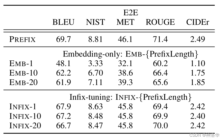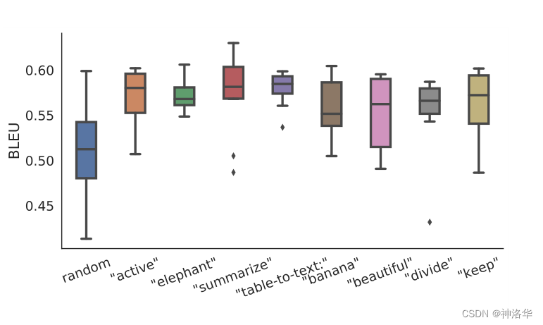
Table 4: Prefix-tuning is better than Embedding-only ablation and Infix-tuning	Figure 5: Initializing prefixes with activations from real words significantly outperforms random initialization when data is scarce.

It can be seen from Figure 5:

• Random initialization results in lower performance and higher variability, initializing the prefix to activations of real words can significantly improve generation
• Initialization with task-related words (such as "summarization" and "table-to-text") performed slightly better than task-independent words (such as "elephant" and "divide")

  Summary: Add the soft prompt represented by Prefix to each layer of the transformer. In order to keep the training stable, it is mapped with the FFN layer before input. Only part of the parameters are updated during training Prefix.

3.2.3 Prompt Tuning（2021.4）

论文《The Power of Scale for Parameter-Efficient Prompt Tuning》

  Prompt TuningIt can be regarded as Prefix Tuninga simplified version of , which defines its own prompt for each task, and then stitches it into the data as input, but only adds prompt tokens in the input layer, and does not need to be adjusted by adding MLP to solve difficult training problems. The pseudo code is as follows:

def soft_prompted_model(input_ids):
	x = Embed(input_ids)
	x = concat([soft_prompt, x], dim=seq)
	return model(x)

The following figure shows the difference between traditional fine-tuning and Prompt Tuning:

• model tuning: Each downstream task undergoes a custom fine-tuning and then maintains a different copy of the pre-trained model, which must be done in separate batches for inference
• Prompt Tuning: You only need to store a small task-specific prompt for each task, and you can use the original pre-trained model for mixed task reasoning
  For the T5 XXL model, each copy of the tuned model requires 11 billion parameters. Prompt Tuning requires only 20,480 parameters per task, a reduction of five orders of magnitude assuming a prompt length of 5 tokens.

  At the same time, Prompt Tuning also proposes Prompt Ensemblingthat different prompts of the same task are trained in a batch (Batch) at the same time (that is, the same question is asked in multiple different ways), which is equivalent to training different models, which is better than model integration. The cost is much less.

  The author performed ablation experiments on both the prompt length and the pre-model size.

Experiment on the T5 model. As the model size increases, Prompt Tuning achieves an effect comparable to full fine-tuning (>10B)

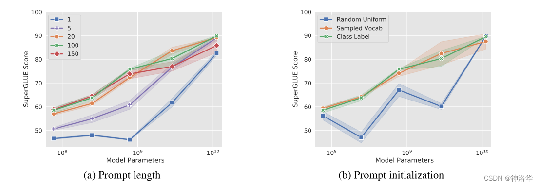
• Prompt length: increasing the length to more than 20 usually improves performance significantly
• The initialization method of prompt, in addition to random initialization, the other two can be used (directly use the category label of the task, or sample vocabulary)
• The size of the model is large enough (>10B), the length of the prompt and the initialization method do not matter

3.2.4 P-tuning (Tsinghua 2022.2)

• Paper "GPT Understands, Too" , code base THUDM/P-tuning
• Refer to Su Shen's "P-tuning: Automatically build templates and release the potential of language models"

3.2.4.1 Principle

  "GPT Understands, Too" proposed a method called P-tuning, which successfully realized the automatic construction of templates. Not only that, with the help of P-tuning, GPT's performance on SuperGLUE surpassed the BERT model of the same level for the first time, which overturned the conclusion that "GPT is not good at NLU" and is also the reason for the name of the paper.

  Intuitively, templates are prefixes/suffixes composed of natural language. Through these templates, we can make downstream tasks consistent with pre-training tasks, make full use of the original pre-training model, and achieve better zero-sample and small-sample learning effects. However, it doesn't care what the template looks like or whether it is composed of natural language, but only cares about the final effect of the model. Therefore, P-tuning considers templates of the following form:

P-tuning directly uses [unused*] tokens to build templates, and does not care about the natural language of templates

  Here [u1]～[u6], it represents the inside of the BERT vocabulary [unused1]～[unused6], that is, unknown tokens are used to form templates . Then, we use the labeled data to find this template. (The number of unknown tokens is a hyperparameter, which can be adjusted at the front or at the back.)

3.2.4.2 Algorithms

1. Template optimization strategy.

   • Labeled data is relatively small : At this point, we fix the weight of the entire model and only optimize [unused1]～[unused6]the Embedding of these tokens. Because there are few parameters to learn, even if there are few labeled samples, the template can be learned, it is not easy to overfit, and the training is fast.
   • Annotated data is sufficient : only optimizing at this point [unused1]～[unused6]will lead to underfitting. Therefore, we can let go of all weight fine-tuning, which is what the original paper's experiments on SuperGLUE did. But what is the difference between this and directly adding a fully connected fine-tuning? The author said that this is better, probably because it is more consistent with the pre-training task.

2. Selection of target tokens
   In the above example, the target tokens such as "sports" are artificially selected, so can they also be replaced by [unused*] tokens? The answer is yes, but there are two situations to consider:

   • When the labeled data is relatively small, it is often better to manually select the appropriate target token
   • When the labeled data is sufficient, it is better to use [unused*] for the target token, because the optimization space of the model is larger at this time.

3. If accessing LSTM
     and initializing the virtual token randomly, it is easy to optimize to a local optimal value, and these virtual token theories should be related (natural language correlation). Therefore, the author encodes these virtual tokens through an LSTM+MLP, and then inputs them into the model. The effect shows that in this way, the model converges faster and the effect is better.

4. Optimization: Target Word Prediction → Sentence Prediction
     Su Jianlin believes that LSTM is to help the tokens of the template (to some extent) be closer to natural language, but this does not necessarily have to be generated by LSTM, and even if it is generated by LSTM, it may not be achieved. at this point. A more natural method is to not only predict the target token of the downstream task (such as "news" in the example) when training the downstream task, but also predict other tokens at the same time.
     Specifically, if it is an MLM model, then randomly mask out some other tokens for prediction; if it is an LM model, predict the complete sequence, not just the target word. Because the models are all pre-trained in natural language, the sequence reconstructed after adding training targets will be closer to the effect of natural language. The author (Su Jianlin) tested and found that the effect has indeed improved.

3.2.4.3 Experimental results

1. The experimental results on SuperGLUE show that both BERT and GPT are P-tuningbetter than BERT Fine-tuning, and the performance of GPT can exceed BERT.
   

   The performance of P-tuning on SuperGLUE, MP means manual prompt.

2. The effect of P-tuning under the language model of each volume
   

3.2.4.4 Comparison of Adapter/Prefix Tuning

• Compared with Adapter: P-tuning is actually a method similar to Adapter. It also fixes the weight of the original model, and then inserts some new optimized parameters, but at this time the new parameters are inserted as templates in the Embedding layer.
• Compared with Prefix Tuning: The differentiable virtual token added by P-Tuning is only limited to the input layer, and it is not added in every layer; in addition, the position where the virtual token is inserted is optional, not necessarily a prefix.

3.2.4.5 Why is it P-tuningbetter thanFine-tuning

  P-tuningand Fine-tuningare fine-tuning all weights, why is it P-tuningbetter than   This is because, whether it is PET or P-tuning, they are actually closer to the pre-training task, and the method of adding a fully connected layer is not so close to the pre-training task, so to some extent, P-tuning is effective It is more "obvious", but it is questionable why adding a fully connected layer fine-tuning is effective.   In the paper "A Mathematical Exploration of Why Language Models Help Solve Downstream Tasks", the author's answer is:Fine-tuning

1. The pre-trained model is some kind of language model task;
2. Downstream tasks can be represented as a special case of this language model;
3. When the output space is limited, it is similar to adding a fully connected layer;
4. So adding a fully connected layer fine-tuning is effective.

  Therefore, PET, P-tuning, etc. are more natural ways to use pre-trained models, and the method of adding full connection and direct finetune is actually just their inference. In other words, PET and P-tuning are the solutions to return to the basics and the essence, so they are more effective.

3.2.5 P-tuning v2 (Tsinghua University 2021.10)

《P-Tuning v2: Prompt Tuning Can Be Comparable to Fine-tuning Universally Across Scales and Tasks》、 thudm/p-tuning-v2

3.2.5.1 Background

  There are two main problems with the previous Prompt Tuning and P-Tuning methods:

1. Lack of versatility.

   • Lack of scale versatility: The Prompt Tuning paper shows that when the model scale exceeds 10 billion parameters, prompt optimization can be comparable to full fine-tuning. But for those smaller models (from 100M to 1B), there is a big difference in the performance of hint optimization and full fine-tuning, which greatly limits the applicability of hint optimization.
   • Lack of task generality: Although Prompt Tuning and P-tuning have shown advantages in some NLU benchmarks, the effectiveness of prompt tuning for hard sequence labeling tasks (i.e., sequence labeling) has not been verified.

2. Missing depth hinting optimizations.
   In Prompt Tuning and P-tuning, the prompt is only inserted into the input embedding sequence of the first layer of the transformer. In the next transformer layer, the embedding of the prompt position is calculated by the previous transformer layer, so:

   • The number of tunable parameters is limited due to sequence length constraints.
   • Input embeddings have only relatively indirect effects on model predictions.

  Considering these problems, the author proposes P-tuning v2to improve Prompt Tuning and P-Tuning as a general solution across scale and NLU tasks, using deep hint optimization (such as: Prefix Tuning).

3.2.5.2 Algorithms

  P-Tuning v2 adds Prompts tokens as input to each layer, instead of just adding it to the input layer, which brings two benefits:

• More learnable parameters: Increased from 0.01% of P-tuning and Prompt Tuning to 0.1%-3%, and it is also efficient enough for parameters.
• Prompt in the deep structure can have a more direct impact on model prediction.

Figure 2: Comparison of P-tuning and P-tuning v2. Orange blocks represent trainable hint embeddings, blue blocks are frozen pretrained model parameters

P-tuning v2 can be regarded as optimized Prefix Tuning:

• Remove reparameterized encoders : Previous methods exploit reparameterization features to improve training speed and robustness (e.g. MLP in Prefix Tuning, LSTM in P-Tuning)). In P-tuning v2, the author found that the improvement of reparameterization is small, especially for smaller models; at the same time, for some NLU tasks, using MLP will reduce performance

• Different prompt lengths for different tasks : The prompt length plays a key role in P-Tuning v2, and different NLU tasks will achieve their best performance with different prompt lengths. In general, easy classification tasks (sentiment analysis, etc.) prefer shorter cues (less than 20 tokens); difficult sequence labeling tasks (reading comprehension, etc.) prefer longer cues (about 100 tokens)
  

  Figure 4: Ablation study of cue length and reparameterization using RoBERTa-large. On specific NLU tasks and datasets, conclusions may vary widely. (MQA: Multiple Choice Question Answering)

• Introduce multi-task learning : pre-train on multi-task Prompt first, and then adapt to downstream tasks. Multitasking can provide better initialization to further improve performance

• Return to the traditional classification labeling paradigm : Label Word Verbalizer has been a core component of hint optimization, which can predict labels in a cloze way. Despite its potential necessity in the few-shot setting, the Verbalizer is not necessary in the full-data supervised setting. It hinders the application of hint tuning in scenarios where we need nonsensical label and sentence embeddings. Therefore, P-Tuning v2 returns to the traditional CLS label classification paradigm, and uses a randomly initialized classification head (Classification Head) to apply to tokens to enhance versatility and can be adapted to sequence labeling tasks.
  

3.2.5.3 Experiment

1. SuperGLUE
   for simple NLU tasks such as SST-2 (single sentence classification), Prompt Tuning and P-Tuning show no significant disadvantages at smaller scales. But when it comes to complex challenges, such as natural language reasoning (RTE) and multiple choice question answering (BoolQ), they perform very poorly. In contrast, P-Tuning v2 matches fine-tuned performance on all tasks at smaller scales.
   Table 2: Results on the SuperGLUE dev set. FT means Fine-tuning, PT and PT-2 mean P-Tuning and P-Tuning v2. The bold type in the figure is the best, and the underline indicates the second best
2. Most of the tasks of the sequence labeling tasks
   GLUE and SuperGLUE are relatively simple NLU problems. In order to evaluate P-Tuning v2the ability in some difficult NLU challenges, the authors selected three typical sequence labeling tasks (named entity recognition, extractive question answering (QA) and semantic role labeling SRL), a total of eight data sets. We observe that P-Tuning v2it is comparable to Fine-tuning.
   

3.2.6 Intrinsic Prompt Tuning (IPT，略)

3.3 Other Approaches（略）