3D Packing for Self-Supervised Monocular Depth Estimation Paper Notes

2019 3D Packing for Self-Supervised Monocular Depth Estimation

1. Basic knowledge:

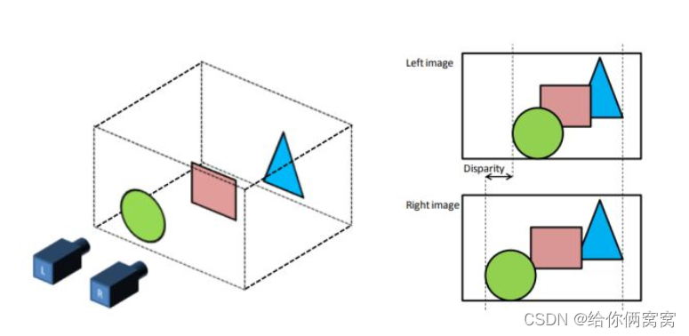
​ As shown in the figure above, although the cameras L and R on the same horizontal plane capture the same object, the pictures generated between them are different, and this difference cannot be eliminated by translating the generated pictures. Objects that are closer to the camera deviate more, and objects that are farther from the camera deviate less. The existence of this difference is brought about by the three-dimensional space. At the same time, the pictures taken by two cameras on the same horizontal line obey the following physical laws:

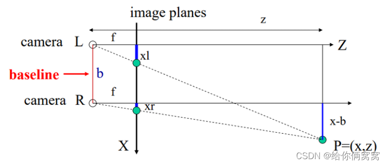
​ In the figure, $z$ is the depth of the scene from us,$X$ is the two-dimensional image plane to which the three-dimensional scene is mapped, that is, the plane where the final two-dimensional image is located. $f$ is the focal length of the camera,$b$ is the distance between the two cameras,$x_l$and $x_r$are the coordinates of the same object imaged by the left and right cameras respectively. According to the above information and the simple triangle similarity rule, we can get:
$$x-b=\frac{z}{f}{x}_r;x=\frac{z}{f}{x}_l;\Rightarrow (x_l-x_r)=\frac{fb}{z}$$
​ Here $x_l-x_r$It is what we often call parallax $d$ (disparity), represents$x_r$This point is in the camera $L$ and cameraRROffset values ​​for imaging in$R.$In other words, this value represents the pixels in the left camera that need to be translated by$d$ to form the corresponding pixel in the right camera. So the relationship between two perspectives can be written as:
$$d=x_l-x_r\Rightarrow x_l=d+x_r$$
​ Suppose we have a very powerful function $F$ , yes this function is a neural network, making$F(I_r)=d$，$I_r$is the image taken by the right camera, then:
$$I_r(x_r)=I_l(x_l);x_l=F(I_r)+x_r;\Rightarrow I_r\left(x_r\right)=I_l(F(I_r)+x_r)$$
​ I$I_l$is the image taken by the left camera, as long as we use $I_l$As input for training, $I_r$As the corresponding reference standard, the neural network $F$ , through the training of a large number of binocular image pairs, the neural network FFobtained$F$ is an input of a picture$I_l$To predict the corresponding disparity $d$ function, so that an unconstrained problem becomes a problem that conforms to the above rules, and it can be solved using conventional thinking. Simultaneous parallax$d$ in known camera parameters$b,In\; the\; case\; of\; f$ , the corresponding depth$z$。

​ Summarizing the above rules, we get: Because monocular depth requires expensive lidar, but the pictures taken by two cameras on the same horizontal line are relatively easy to obtain. As long as we obtain the corresponding disparity $d$ , while knowing the camera parameters$(b,In\; the\; case\; of\; f)$ , the corresponding depth$z$。

​ Through the above, the monocular depth estimation problem can be written as a simple function:
$$z=\frac{fb}{d};d=F(I_r);\Rightarrow z=fb\frac{1}{F(I_r)}$$
​ That can be written as:
$$z=F\left(I\right)$$
​ zz$z$ is the predicted depth,$d$ is the parallax under fixed camera,$b$ is the distance between the two lenses of the camera,$f$ is the focal length.

​ We know that $z=F\left(I\right)$ This relationship can be easily simulated using CNN, but there is a problem, the$d$ is a continuous floating point number, if you use$x_l-d$ routine, then it is likely to fall into a position that is not in the (integer) pixel point, and at the same time due to different positions$d$ is different, it is also possible to have an$I_r$Pixels in $x_r$Accept multiple from $I_l$because they all satisfy $x_r=x_{l_1}-d_1=x_{l_2}-d_2=x_{l_3}-d_3...$ . **And there are some points that do not match$d$ , because these points may not be visible at all in the original image due to parallax. **In order to solve this problem, the method of backward (reverse) mapping is generally adopted, as shown in the following figure:

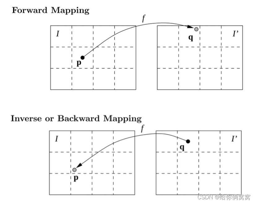
​ The difference between these two methods is that in forward mapping, we get $I^{’}$ may fall on a position that is not an integer pixel point, at this time, the original imageIIThe pixels in$I$$I^{\prime }$ ; and in Inverse mapping, we start from$I^{\text{'}}$ Departure (that is,$x_r+d$ ), to find the corresponding points in the original image, so as to ensure$I^{\prime }$ has assignments without holes, and if$x_r+$The points in the original image obtained by$d$ do not belong to (integer) pixel points. At this time, the position of the corresponding non-pixel point can be obtained by interpolationmethod. Generally, bilinear interpolation method is used here, and it is in sub-pixel The level is guided [Spatial Transformer Networks], so that the network can be trained end-to-end.

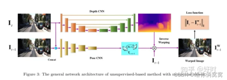
​ During training, our network is divided into the following steps:
$$d=F(I_r)$$

$$I_l^{\prime }=Mapping(I_r,d)$$

​ And the corresponding loss function is:
$$argmi{n}_{}Loss(I_l^{\prime },I_l)So\; far$$
, the forward propagation process passes$F$ to get the corresponding parallax$d$ ,the mapping process converts the left image into the right image, the loss function calculates the current accuracy and enters the optimization process, the backpropagation process is described as follows:
$$\frac{\delta Loss}{di}=\frac{\delta Loss}{\delta mapping}\times \frac{\delta mapping}{F\_}\times \frac{F}{di}$$
​ In the above formula, $\theta$ isFFThe parameters of the neural network to be optimized in$F$$\frac{\delta Loss}{\delta mapping}$Obtained by the loss function, $\frac{\delta mapping}{F\_}$Default mapping, $\frac{F}{di}$It is obtained by backpropagating the neural network itself. The test process only requires $I$ pass into the neural network$F$ can get the corresponding parallax, combined with the camera parameters, you can get the depth.

2. Basic network:

3. Innovation points:

1) A new convolutional network architecture, called PackNet , is proposed for high-resolution self-supervised monocular depth estimation. The authors propose new compression and decompression blocks that jointly leverage 3D convolutions to learn representations that maximize the propagation of dense appearance and geometric information, while still being able to run in real-time. 2) A new loss is proposed that is able to exploit the speed of the camera to resolve the scale ambiguity inherent in monocular vision. 3) Propose a new dataset : Dense Deep for Autonomous Driving (DDAD) dataset. It utilizes various logs from a well-calibrated fleet of autonomous vehicles equipped with cameras and high-precision long-range LiDAR. Compared with existing baselines, DDAD enables more accurate depth estimation over a range of distances, which is crucial for high-resolution monocular depth estimation methods.

4. The overall network structure of the paper:

Figure 2: PackNet-SfM : The author's scale-aware self-supervised monocular motion structure architecture. We introduce PackNet as a new deep network and optionally include weak velocity supervision at training time to produce scale-aware depth and pose models.

5、PackNet：

Standard convolutional architectures use large strides and pooling to increase the size of their receptive fields. However, this may degrade model performance for tasks that require fine-grained representations [20, 50]. Likewise, traditional upsampling strategies [12, 7] fail to propagate and preserve enough details at the decoder layer to recover accurate depth predictions. In contrast, the authors propose a novel encoder-decoder architecture called PackNet, which introduces new 3D compression and decompression blocks to learn to jointly preserve and recover important spatial information for depth estimation. The authors first describe the different blocks of the proposed architecture and then go on to show how they are integrated in a single model for monocular depth estimation.

5.1. Compression block:

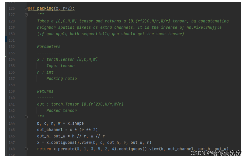
The compression block (Fig. 3a) first collapses the spatial dimensions of the convolutional feature maps into additional feature channels via the Space2Depth operation [40]. The resulting tensor has reduced resolution, but this conversion is reversible without any loss compared to striding or pooling. Next, learn to compress this concatenated feature space to reduce its dimensionality to the desired number of output channels. As demonstrated by the ablation experiments, 2D convolutions are not designed to directly exploit the tiled structure of the feature space.

Figure 3: Proposed 3D compression and decompression blocks. Compression replaces striding and pooling, while decompression is an upsampling mechanism for its symmetric features

Instead, the authors propose to first learn to extend this structured representation through 3D convolutional layers. The resulting high-dimensional feature space is then flattened (by simple reshaping) before the final 2D convolutional shrinking layer. This structured feature expansion contraction inspired by reversible networks [22, 4], although the authors do not ensure reversibility, allows the architecture to invest more parameters to learn how to compress the key spatial details that high-resolution deep decoding needs to preserve.

5.2. Decompress the block:

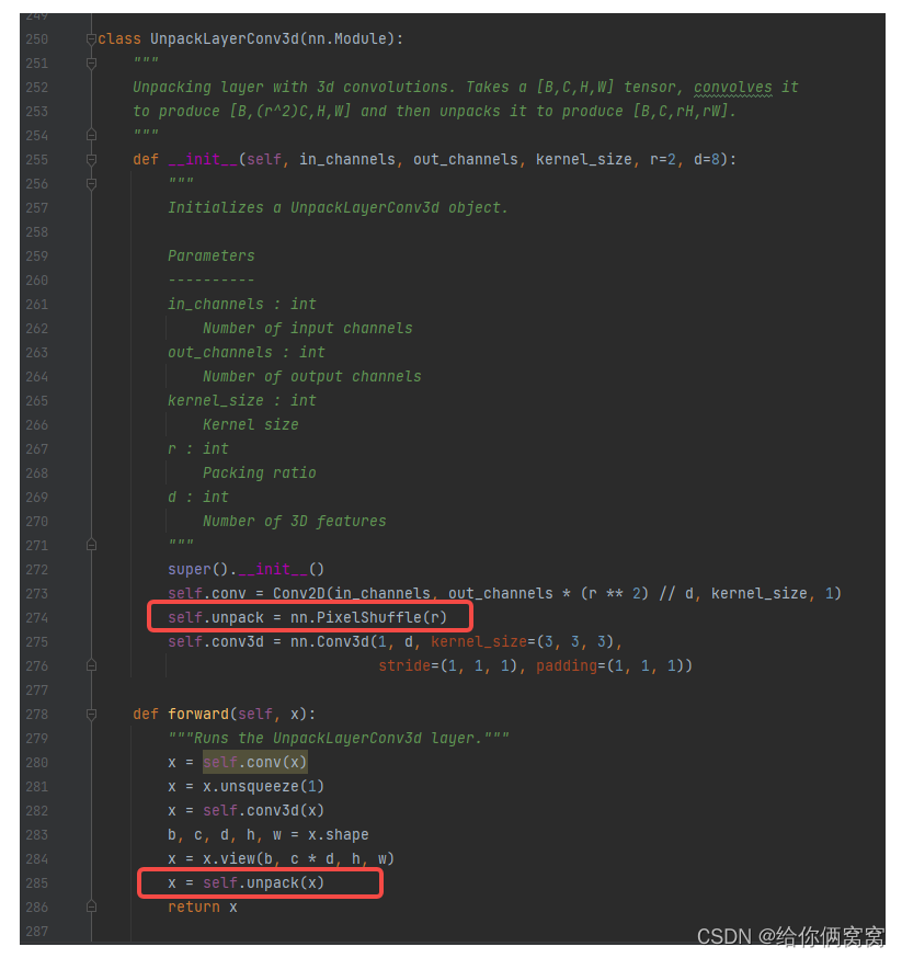
Symmetrically, the decompression block (Fig. 3b) learns during decoding to decompress and expand the compressed convolutional feature channels back to higher resolution spatial dimensions. The decompression block replaces convolutional feature upsampling, usually performed by nearest-neighbor or learnable transposed convolutional weights. It is inspired by sub-pixel convolution [40] but adapted to invert the 3D compression process of features in the encoder. First, the authors use 2D convolutional layers to generate the required number of feature channels for subsequent 3D convolutional layers. Second, this 3D convolution learns to expand compressed spatial features. Third, these decompressed features are converted back to spatial details via reshape and Depth2Space operations [40] to obtain tensors with the desired number of output channels and higher resolution targets.

5.3. Results of image reconstruction using PackNet:

In Figure 4, the authors illustrate the detail-preserving properties of the compression/decompression combination, showing that $L_1$loss to obtain a nearly lossless encoder-decoder for single image reconstruction. The authors train a simple network consisting of a compression layer followed by a symmetric decompression layer, and show that it can reconstruct an input image almost accurately (final loss 0.0079), including sharp edges and finer details. In contrast, comparable baselines that replace compression/decompression with max pooling/bilinear upsampling (and keep 2D convolutions) can only learn blurry reconstructions (final loss of 0.063). This highlights how PackNet is able to learn more complex features by preserving spatial and appearance information end-to-end throughout the network.

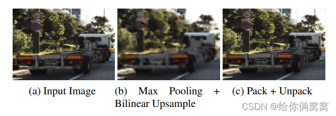
Figure 4: Image reconstruction with different encoder-decoders: (b) standard max pooling and bilinear upsampling, each followed by 2D convolution; © $D=2$ a combination of compression and decompression (see Figure 3). For the middle channel, all kernel sizes are$K=3$ and$C=4$

5.4, ​​PackNet model structure:

Table 1 details the author's PackNet structure for self-supervised monocular depth estimation. The symmetric encoder-decoder structure proposed by the authors consists of multiple compression and decompression blocks, supplemented by skip connections [36] to facilitate the flow of information and gradients throughout the network. The decoder generates intermediate inverse depth maps, which are upsampled before being concatenated with corresponding skip connections and decompressed feature maps. These intermediate inverse depth maps are also used for loss computation at training time after upsampling to the full output resolution using nearest neighbor interpolation.

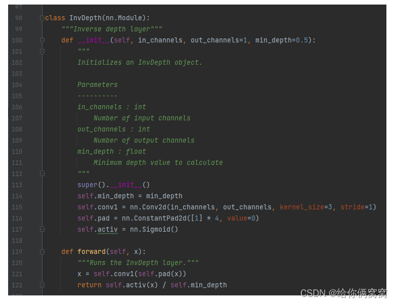
Table 1: Summary of PackNet architectures for self-supervised monocular depth estimation . The Packing and Unpacking blocks are shown in Figure 3, the kernel size $K=3$ and$D=8$ . The Conv2d block includes Group-Norm [46] with G=16 and the ELU non-linear activation function [8]. The InvDepth block contains a$K=3$ and sigmoid nonlinear 2D convolutional layers. Each ResidualBlock is a sequence of 3 2D convolutional layers,$K=3/3/1$ and ELU nonlinear activation function, the last layer is$G=GroupNorm\; of\; 16$ and Dropout of 0.5 scale [41]. Upsample is the nearest neighbor interpolation operation. Numbers in parentheses indicate input layers, + are connected as channels.

6. Loss function:

$$L_{scale}(I_t,{\hat{I}}_t,v)=L(I_t,{\hat{I}}_t)+l_2{L}_v({\hat{t}}_{t->s},v)$$

$$L_p(I_t,I_S)=mi{n}_{I_S}{L}_p(I_t,{\hat{I}}_t)$$

$$L_p(I_t,{\hat{I}}_t)=a\frac{1-SSIM(I_t,{\hat{I}}_t)}{2}+(1-a)||I_t-{\hat{I}}_t||$$

$$M_p=mi{n}_{I_S}{L}_p(I_t,I_s)>mi{n}_{I_S}{L}_p(I_t,{\hat{I}}_t)$$

$$L_s({\hat{D}}_t)=|{\delta }_x{\hat{D}}_t|e^{-|{\delta }_x{I}_t|}+|{\delta }_y{\hat{D}}_t|e^{-|{\delta }_y{I}_t|}$$

​ Among them, $I_t$is the target image, ${\hat{I}}_t$is the synthetic target image, $L_p$is the appearance matching loss, $I_S$Is $I_s$The collection of , the context view, $I_s$is the source image, the original $L_p$There will be a parallax effect in the middle, in order to eliminate the parallax effect, calculate $I_S$L p L_p of each picture in$L_p$Then take the smallest as the new $L_p$ 、$M_p$is an automatic mask that removes pixels that do not change in appearance between frames, including static scenes and dynamic objects without relative motion. When assuming no self-motion, their luminosity loss is small, M t $M_t$is a binary mask that does not count pixels of the source image that are not projected onto the target image given the estimated target depth, $\lambda$ ₁is the depth regularization term,$L_s$is the depth smoothing loss, ${\hat{D}}_t$Is the depth estimation, in the area where the texture is not obvious/low resolution, the estimated depth ${\hat{D}}_t$The regularized smoothing term for , decays according to the sampling rate weight.
$$L_v({\hat{t}}_{t->s},v)=|||{\hat{t}}_{t->s}||-|v|\Delta T_{t->s}|$$
​ During the training process, calculate the size of the pose translation component predicted by the pose network$\hat{t}$ and the measured instantaneous velocity scalar$v$ is multiplied by the time difference between the target frame and the source frame$\Delta T_{t->s}$, and an additional loss L v L_v is imposed between$L_v$。

7. Proposed new dataset:

​DDAD (Dense Depth for Automated Driving) . The authors publish a diverse dataset of urban, highway, and residential scenarios curated by fleets of autonomous vehicles around the world. It contains 17,050 training frames and 4,150 evaluation frames, as well as ground-truth depth maps generated from dense LiDAR measurements using the Luminar-H2 sensor. This new dataset is a more realistic and challenging benchmark for depth estimation because it is diverse and can capture cross- The exact structure of the image. (30k points per frame).

8. Implementation details:

The authors train all models on 8 Titan V100 GPUs using Pytorch. Use Adam optimizer, where $b_1=0.9$、$b_2=0.999$ . The monocular depth and pose network is trained for 100 cycles, the batch size is 4, and the initial depth and pose learning rates are$2\cdot 10^{-4}$ and$5\cdot 10^{-4}$ .${}^{\_}$The training sequence is generated using stride 1, which means using$t-1$ frame, current frame$t$ and$t+1$ frame to calculate the loss. As training progresses, the learning rate decays by a factor of 2 every 40 epochs. The author sets the SSIM weight to$a=0.85$ , the depth regularization weight is set to$l_1=0.001$ , and where available, the velocity scaling weight is set to$l_2=0.05$。

​Deep Web . Unless otherwise stated, the authors use the PackNet structure specified in Table 1. During training, all 4 inverse depth output scales are used for loss computation. When testing, only the final output scale is used after resizing the full-truth depth map resolution using nearest neighbor interpolation.

​Pose network . The authors use the structure proposed by [52] without the interpretability mask and find that it does not improve the results. The pose network consists of 7 convolutional layers and a final 1x1 convolutional layer. The input to the network is represented by the target view $I_t$and the context view $I_S$Composition, the output is $I_t$Sum $I_s$A set of 6-DOF transformations between , where $s\in S$。

9. Experimental results:

First of all, due to the introduction of the new DDAD dataset, the monocular depth estimation method proposed by the author considers the performance at longer distances. Depth estimation results for training and testing using this dataset, considering cumulative distances up to 200 m, can be found in Fig. 5 and Table 2.

Figure 5: PackNet point cloud reconstruction on the DDAD dataset

Table 2: Depth tests on the DDAD dataset , 640x384 resolution and up to 200m distance. While the ResNet family of validation relies on massively supervised ImageNet pre-training (denoted by ‡ ), significantly better results are achieved when PackNet is trained from scratch.

Furthermore, in Figure 6, the authors show the results for different depth intervals calculated independently. As can be seen from these results, the PackNet-SfM approach significantly outperforms the state-of-the-art [19] based on the ResNet family, and the performance gap continues to increase when larger distances are considered.

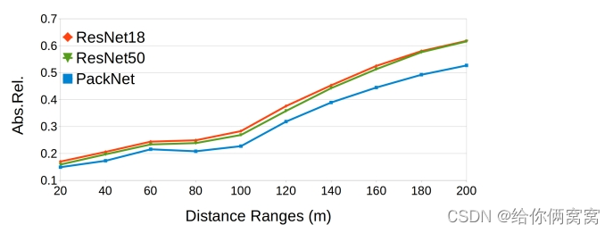
Figure 6: Depth evaluation for binning DDAD at different intervals, independently computed by only considering ground-truth depth pixels in this range (0-20m, 20-40m, ...).

Second, the authors evaluate KITTI's depth prediction using the metrics described in Eigen et al. [14]. For raw depth maps from [14] and cumulative depth maps from [42], the results are summarized in Table 3 and their performance is qualitatively illustrated in Fig. 7. Compared with previous methods [6, 19], which mainly focus on modifying the training objective, it is shown that the authors' proposed PackNet structure can improve performance by itself and establish a new state-of-the-art for the monocular depth estimation task, in a self-supervised monocular training environment.

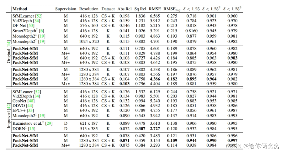
Table 3: Quantitative performance comparison of PackNet-SfM on the KITTI dataset for distances up to 80m. For Abs Rel, Sq Rel, RMSE and RMSElog the lower the better, for $d<1.25$、$d<1.252$和$d<1.253$ The higher the better. In the Dataset column, CS+K refers to pre-training on CityScapes (CS) and fine-tuning on KITTI (K). M refers to the method of training using monocular images, and M+v refers to adding speed weak supervision, see Section 3.2. ‡ Refers to pre-training on ImageNet. Original is evaluated with raw depth maps from [14], while Improved uses annotated depth maps from [42]. During the testing phase, all monocular methods use intermediate ground-truth LiDAR information to estimate depth. The Velocity-scaled (M+v) and supervised (D) methods are not scaled in this way because they are already metered.

Figure 7: Qualitative monocular depth estimation performance comparison of PackNet with previous methods on frames from the KITTI dataset (Eigen test split). Due to the learned preservation of spatial information, our proposed method is able to capture sharper details and structures (e.g., vehicles, pedestrians, and thin poles).

Furthermore, the authors show that monocular depth estimation performance can be further improved by simply introducing additional unlabeled video sources, such as the publicly available CitySpaces dataset (CS+K) [9]. As pointed out by Pillai et al. [39], the authors also need to observe an increase in performance at higher image resolutions, which the authors attribute to the fact that the proposed network correctly preserves and processes spatial information end-to-end. The best results in this paper are achieved when training with more unlabeled data injected and higher resolution input images, and the performance is comparable to semi-supervised [29] and fully supervised [15] methods.

In Table 6, the authors show the results of the PackNet SfM framework on the KITTI benchmark. For comparison with related methods, the authors train on sequences 00-08 of the KITTI benchmark, using exactly the same parameters and networks as in Table 3 in the main text. In keeping with related methods, we compute the average absolute trajectory error (ATE) for all overlapping 5-frame clips on sequences 09 and 10. Note that our pose network takes only two frames as input and outputs a single transformation between the pair of frames. To evaluate our model on 5-frame fragments, we combine the relative transition frames between the target frame and the first context into 5-frame long overlapping trajectories, i.e. we stack fx ( I t , I t − 1 = xt − $f_x(I_t,I_{t-1}=x_{t->t-1})$ to create an appropriately sized trajectory.

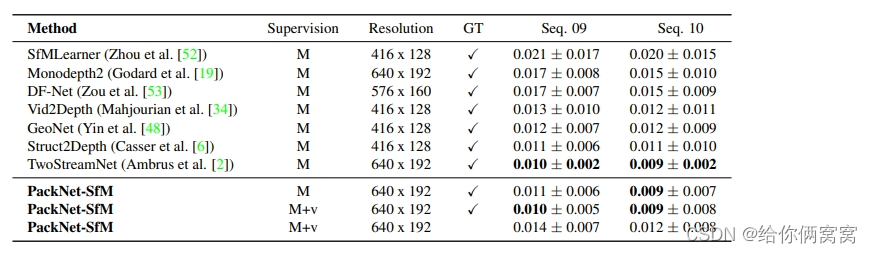
Table 6: Mean absolute trajectory error (ATE) in meters on the KITTI odometry benchmark [17] : All methods are trained on sequence 00-08 and evaluated on sequence 09-10. The ATE number is the average of all overlapping 5-frame segments in the test sequence. In addition to monocular images (M), M+v refers to velocity supervision (v). A GT check mark indicates that the estimate at test time is scaled using the ground truth transformation.

ATE results are summarized in Table 6, and the authors' proposed framework achieves competitive results compared to other related methods. The authors also note that all these related methods are trained in the monocular setting (M) and thus use ground truth information for scaling at test time. On the other hand, the velocity supervision loss (M+v) proposed by the authors does not require ground-truth scaling at test time for training, since it fully recovers the metric-accurate scale from monocular images. Nevertheless, it can still achieve competitive results compared with other methods. An example of reconstructed trajectories obtained for the test sequence using PackNet-SfM can be found in Figure 9.

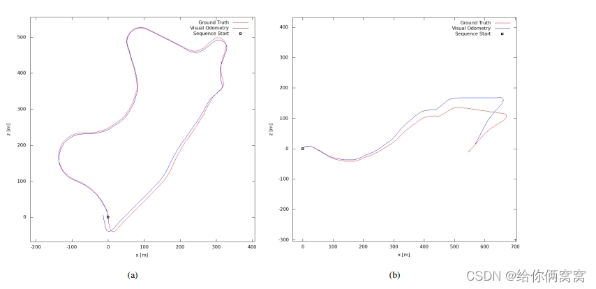
Figure 9: Pose evaluation for the KITTI test sequence . Qualitative trajectory results of PackNet-SfM on KITTI odometry benchmark sequences 09 and 10.

10. Network complexity:

Introducing compression and decompression as an alternative to standard downsampling and upsampling operations increases the complexity of the network due to the increased number of parameters. To ensure that the performance gains shown in the experiments are not simply due to increased model capacity, the authors compared different variants of the PackNet structure (obtained by modifying the number of layers and feature channels) with the ResNet structure. These results, shown in Figure 8, show that while the ResNet family is stable with diminishing returns as the number of parameters increases, the PackNet family matches its performance at around 70M parameters and improves further with increasing complexity. Finally, the proposed structure (Table 1) achieves about 128M parameters and 60ms inference time on a Titan V100 GPU, which can be further improved to <30ms using TensorRT, making it suitable for real-time applications.

Figure 8: Performance of different deep network architectures with different numbers of parameters on the original KITTI Eigen split [14] at resolutions 640 x 192 (MR) and 1280 x 384 (HR) . While the ResNet series is stable at 70M parameters, the PackNet series matches its performance at the same number of parameters for MR, significantly outperforms it in HR, and does not overfit as parameters increase.

The PackNet family also performs consistently better at higher resolutions, as it appropriately preserves and propagates spatial information between layers. In contrast, as illustrated in a previous paper [19], the ResNet architecture does not scale well, with only marginal improvements at higher resolutions.

11. Ablation experiment:

In order to further study the performance improvement provided by PackNet, the authors conducted ablation experiments on the different structural components introduced, as shown in Table 4. The authors show that, without proposing compression and decompression blocks, the basic structure already yields a strong baseline for the task of monocular depth estimation. The introduction of compression and decompression improves depth estimation performance, especially when adding more 3D convolutional filters, and the structure described in Table 1 achieves state-of-the-art results.

Table 4: Ablation studies of the PackNet architecture on the standard 640x192 resolution KITTI benchmark. ResNetXX indicates a specific structure [21] as an encoder, and ‡ indicates that ImageNet was used for pre-training. The authors also show the results of the proposed PackNet structure, first removing compression and decompression (replaced by convolutional striding and bilinear upsampling, respectively), and then increasing the number of 3D convolutional filters (D=0 means no 3D convolution).

As mentioned in [19, 15], ResNet architectures benefit greatly from ImageNet pre-training since they were originally developed for classification tasks. Interestingly, the authors also note that the performance of pretrained ResNet architectures degrades over longer training epochs due to catastrophic forgetting that leads to overfitting. On the other hand, the proposed PackNet architecture achieves state-of-the-art results from randomly initialized weights, and can be further improved by self-supervised pre-training on other datasets, thus due to its structure, can properly exploit unlabeled information. Availability at scale.

12. Generalization ability:

The authors also study the generalization ability of PackNet as evidence that it does not just memorize the training data but learns transferable discriminative features. To evaluate this, the authors test models on the recently released NuScenes dataset, which were trained on a combination of CitySpaces and KITTI (CS+K), without any fine-tuning. The results are shown in Table 5:

Table 5: Generalization capabilities of networks of different depths , trained on KITTI and CitySpaces and tested on NuScenes at a resolution of 640x192 at distances up to 80m. ‡ indicates pre-training on ImageNet.

PackNet does generalize better on countries with a large number of vehicles (CS+K in Germany, NuScenes in the US+Singapore), outperforming standard architectures on all metrics considered without requiring Perform large-scale supervised pre-training.

code:

GitHub - TRI-ML/packnet-sfm: TRI-ML Monocular Depth Estimation Repository

Reference link:

https://blog.csdn.net/rocking_struggling/article/details/105470845 (PixelShuffle)

https://blog.csdn.net/qq_34745941/article/details/127748132(⊙)

https://zhuanlan.zhihu.com/p/29968267