Paper address: 3D human pose estimation in video with temporal convolutions and semi-supervised training
Code address: VideoPose3D
Paper summary
The method in this paper is called VideoPose3D and uses 2D key point sequence ( xi, yi x_i, y_ixi,andi) Predicting the 3D key points at a certain time point is roughly using a 2D coordinate sequence (rather than acting on the 2D heatmap) action to fit a point with depth. During training, this paper also proposes a simple but effective semi-supervised method to use video data that is not unlabeled. The semi-supervised method roughly predicts the unlabeled 2D video first, then estimates the 3D pose, and maps the 3D key points to the input 2D key points through the post-mapping.
If only coordinate prediction is performed, the predicted 3D coordinate will always be fixed at the center of the screen. If you need to change the task, you need to predict another root node trajectory. Root node trajectory regression and 3D joint point review will affect each other, so there is no shared network .
Introduction
Concept introduction
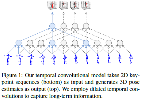
Turning 3D detection into 2D+3D, although reducing the difficulty of the detection task, is also vague and ambiguous in nature. Because multiple 3D points correspond to 1 2D point in the image. A rough diagram of the model structure is shown in the figure below, using hole-time sequential convolution to obtain long-term information. Finally, models that use supervised learning and models that use semi-supervised learning are superior to the most advanced models at the time that use additional data.
In the paper, an important point is put forward: in the two-step 3D detection method, the difficulty lies in predicting an accurate 2D pose, while predicting 3D from ground-truth is relatively simple. Therefore, the author proposes to train a cpn-ResNet50 to predict 2D pose instead of directly using ground truth, which greatly reduces the generalization error of training and training in reality, thereby improving the actual use ability.
In related work, another point of view: The 2D input sequence is as long as the 3D output sequence, which will allow a deterministic conversion of 2D and is a more natural choice.
Model design
The model result of VideoPose3D is shown in the following figure: For J joint points (x, y) (x,y)(x,y ) Yes, apply time domain convolution, convolution kernel size W, channel C. Then add B ResNet-Style blocks. For each block, add a 1D conv first, kernel_size isWWW , the hole convolution factorD = WBD=W^BD=WB , add another1 ∗ 1 1*11∗1 conv/BN/ReLU/Dropout. The last output layer predicts the 3D points of all frames to utilize the temporal information of past and future data. The size of the first convolution kernel of each blockWWW and void factorDDD should be set to the size of the receptive field that can cover all input frames.

In a real-time scene, causal convolution is used, and the model structure is shown in the following figure: only the past frame sequence is used, and future frames are not applicable.

In image convolution, the input and output sizes are generally the same with zero-padding. However, experiments have shown that using boundary frames to fill the input sequence will give better results.
Semi-supervised method
Using semi-supervision can improve accuracy. The author uses the encoder to predict the 2D joint point coordinates to 3D, and then uses the decoder to map the 3D pose back to the 2D coordinates, so that the data without 3D coordinates can be used for training, and the 2D coordinates and the 2D coordinates mapped back by the decoder are used for punishment training.
The author proposes a method of using supervision and semi-supervision together. The first half is supervised learning, and the second half is semi-supervised learning to see if the 3D mapping back to 2D is consistent with the input. The training method is shown in the figure below.

If there is no global position, the predicted 3D object will always be projected in the center of the screen at a fixed scale. Trajectory regression and 3D regression will affect each other, so there is no shared network. The loss function of the trajectory is shown in the following formula: E = 1 yz ∥ f (x) − y ∥ E=\frac1{y_z}\|f(x)-y\|E=andfrom1∥f(x)−y ∥ is expressed as a weighted MPJPE.
The return of a long target trajectory is not particularly important to our task. Because when the object is far away, the trajectory is relatively concentrated.
Semi-supervised learning, in order to make the network more than just assign input. So the author added soft constraints to approximate the bone length of the unmarked batch target and the bone length of the marked batch target. This is important for self-monitoring. So added bone length L2 loss.
Network details
2D pose
The 2D pose used in this article is CPN + Mask RCNN, in which Mask RCNN uses ResNet101 as the backbone.
Mask RCNN and CPN are pre-trained on the COCO data set, and then finetune is performed on the 2D mapping of Human3.6M to better adapt to the data set (there is also corresponding ablation learning, the CPN learned by COCO is directly in Human3.6M 3D prediction training on the data set).
Because the 2D keypoint of human3.6M is different from COCO, when performing finetune on Human3.6M, it is necessary to reinitialize the last layer and add another layer of deconv to return to the heatmaps to learn the new keypoint.
3D pose
Under normal circumstances, global trajectory prediction is not performed unless semi-supervised learning is used.
In the training of the preliminary experiment, the author found that a large number of adjacent frames are worse than not using time domain information (batch of random samples). Therefore, the author chose to cut out the response clips from different videos and mix them for training.
In terms of experimental details, it was found that stride's conv can be used to replace dilation conv to optimize a single frame. During inference, the entire sequence can be processed and the intermediate states of other 3D frames can be reused to improve the inference speed. During training, it is found that if the BN parameter is trained with the default value, it will cause the test error to fluctuate greatly ( ± 1 \pm1± 1 mm). Therefore, the parameter attenuation strategy of the BN layer is set: Initially,β = 0.1 \beta=0.1b=0 . . 1 , exponential decay toβ = 0.001 \ beta = 0.001b=0 . 0 0 1 . Finally, during testing, a flip operation was added.
Experimental results
Timing dilation conv model
The table below shows the comparison with other advanced models. The model in this paper has the lowest average error at the time under all standards, and does not depend on other data. It should be noted that the model clearly uses the timing information, so it is 5mm lower than the single-frame experiment on MPJPE. But the single frame model is also better than others. It should also be noted that the model in this table is obtained by 2D sequence training of CPN after finetune, not ground_truth .

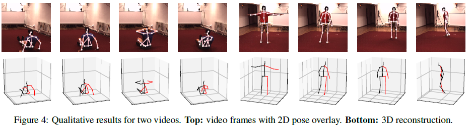
The above timing dilation conv uses the information of past and future frames. If you need to perform 3D prediction in a real-time scene, you need to use casual conv, which will predict the 3D pose of the last frame. The partial display results of the dilation conv timing model are shown in the following figure.
Interestingly, the performance of using Mask RCNN and ground-truth bounding box is similar, which means that the detection result is almost perfect in this single-person scene.
The following table shows the influence of the sequence predicted by the 2D points on the 3D pose, which shows the results of various 2D sources. The improvement of CPN & Mask RCNN display results may be higher heatmap resolution, stronger feature merging, or more discrete pre-training data set.

The absolute position error cannot measure the smoothness of the prediction. And smoothness is very important for video. To evaluate this, the joint velocity error (MPJVE) is used, which corresponds to the first derivative of the 3D sequence of MPJPE. Table 2 shows that the timing model reduces the MPJVE single frame baseline by an average of 76%, thus greatly smoothing the 3D pose.

The following table shows the results of training on the HumanEva-I dataset.

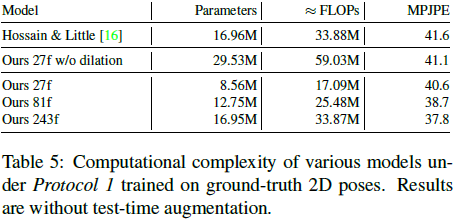
The following table compares the complexity of CNN and LSTM, and also compares the results of 3D pose estimation using 2D sequences of different lengths.