Random Forest Principle and Performance Analysis

Getting Started with Random Forests

Decision trees are described in detail in Introduction to Decision Trees, sklearn Implementation, Principle Interpretation and Algorithm Analysis , but only one decision tree is considered. As the saying goes, among the three cobblers, the best is Zhuge Liang. This article will study how to further improve the effect of the model by combining multiple decision trees, that is, random forest.

In order to understand the principle behind the random forest algorithm, let's first look at a very simple but very interesting example: there are 3 judges who need to judge whether the defendant is guilty, and the final judgment result is determined by a minority obeying the majority.

Assume that the probability of each judge being correct is $p$ , if there is only one judge, then the probability that the judge is correct is$p$。

When the number of judges increases to 3, there are two situations in which the final judgment can be correct: one is that all three judges are correct, and the other is that only one judge is wrong and the other two are correct. Its total probability is
$$p^3+3p^2(1-p)$$

It makes sense to increase the number of judges only when the probability of 3 judges being correct is higher than the probability of 1 judge being correct. At this time,
$$p^3+3p^2(1-p)>$$
Simplify$$p$$
$$p(p-1)(p-0.5)<0$$
because$The\; basic\; constraints\; of\; p$ are$0\le p\le 1$ , combined with the above formula, the constraints can be changed to
$$0.5<p<1$$

That is to say, as long as the probability of correct judgment of unit judges exceeds 0.5, increasing the number of judges can further increase the probability of correct judgment.

In addition to the probability constraints, two other constraints are implied in the above derivation process: (1) The judges make independent judgments independently of each other, which is the basic premise for calculating the probability of the correct judgment of the three judges; Voting objects have a common purpose, because if a judge deliberately shields a criminal, he may deliberately give a wrong judgment.

In fact, there is already a theorem describing this situation, the Condorcet jury theorem: An odd number of people (models) classify an unknown world state as true or false. The probability of each person (model) being correctly classified is $p>0.5$ , and the probability that any one person (model) is classified correctly is statistically independent of the correctness of the classifications of other people (models). The theorem can be described as: the probability of the majority vote being correct is higher than that of any person (model); when the number of people (model number) becomes large enough, the accuracy rate of the majority vote will be close to 100%.

Construct Random Forest

Apply the Condorcet jury theorem to the random forest algorithm: as long as the multiple trees are independent of each other and the probability of each tree predicting correctly exceeds 0.5, the effect of the random forest algorithm can be better than that of a single decision tree.

The correct probability of a single decision tree prediction is more than 0.5, because the correct probability of random guessing is already 0.5. After learning the training set, it can be expected that the probability of correct judgment exceeds 0.5.

The way to make multiple trees independent of each other is:
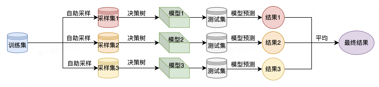
(1) Generate different and independent data sets through the bootstrap sample strategy. The specific process is as follows: Repeated random sampling of a sample from the original data set with replacement (that is, the same sample can be drawn multiple times), the number of extractions is the same as the number of original data sets, which will create a data set with the same size as the original data set set, but some data points will be missing (about 37%), and some will be repeated.
(2) Construct a decision tree based on the newly created dataset, but with a slight modification of the algorithm we described in the introduction to decision trees . At each node, the algorithm randomly selects a subset of features and finds the best test for one of the features, rather than finding the best test for every node. The number of features selected is controlled by the max_features parameter. The selection of a subset of features at each node is independent of each other, so that each node of the tree can use a different subset of features to make a decision.

Due to the use of bootstrap sampling, each decision tree in a random forest is constructed from a slightly different dataset. Due to feature selection at each node, each split in each tree is based on a different subset of features. Together, these two steps ensure that all trees in the random forest are unique and independent of each other.

To make predictions using random forests, you first need to make predictions for each tree in the forest. Thereafter, for the regression problem, we average these results as the final prediction. For classification problems, a "soft voting" strategy is used. That is, each algorithm makes a "soft" prediction, given the probability of each possible output label, averages the predicted probabilities across all trees, and takes the class with the highest probability as the prediction.

The following is a flow chart when using random forests to solve forecasting problems.

Random Forest Performance

Let's first look at the results of random forest and each decision tree through visualization. The following is the implementation code using the sklearn package.

import mglearn.plots
from sklearn.ensemble import RandomForestClassifier
from sklearn.model_selection import train_test_split
import matplotlib.pyplot as plt

from data import two_moons


if __name__ == '__main__':
    X, y = two_moons.two_moons()
    # 数据集拆分
    X_train, X_test, y_train, y_test = train_test_split(X, y, random_state=0)
    # 创建一个随机森林分类器，包含 5 棵树，随机种子为 2
    forest = RandomForestClassifier(n_estimators=5, random_state=2)
    # 使用训练数据拟合模型
    forest.fit(X_train, y_train)

    # 创建一个 2x3 的图像，用于显示每棵树的分割情况
    fig, axes = plt.subplots(2, 3, figsize=(20, 10))
    # 遍历每棵树，显示其分割情况
    for i, (ax, tree) in enumerate(zip(axes.ravel(), forest.estimators_)):
        ax.set_title('Tree {}, score {:.2f}'.format(i, forest.estimators_[i].score(X_train, y_train)))
        # 绘制决策树
        mglearn.plots.plot_tree_partition(X_train, y_train, tree, ax=ax)

    # 在最后一个子图中显示整个随机森林的决策边界
    mglearn.plots.plot_2d_separator(forest, X_train, fill=True, ax=axes[-1, -1], alpha=0.4)
    axes[-1, -1].set_title('Random Forest, , score {:.2f}'.format(forest.score(X_train, y_train)))
    # 在前两个子图中显示训练数据的散点图
    mglearn.discrete_scatter(X_train[:, 0], X_train[:, 1], y_train)

After running the code, you can get the following figure. The results of the random forest model are visually superior to individual decision trees. From the score point of view, the values ​​of the five decision trees are 0.88, 0.93, 0.93, 0.95 and 0.84 respectively, while the random forest further improves the score to 0.96.

Calculating feature importance is much simpler, just one line of code:

forest.feature_importances_

The following is the output

array([0.38822127, 0.61177873])

When using a single decision tree to solve, we mentioned at the time that the importance values ​​were 0.1478 and 0.2138, respectively.

It seems that the difference is quite large, but it is actually because the importance value was not normalized at that time. After normalization, the importance value of the first feature is:
$$0.1478/(0.1478+0.2138)=0.4087$$
The importance value of the second feature is:
$$0.2138/(0.1478+0.2138)=0.5913$$
Now it seems that the difference under the two methods is not that big.

Random Forest Characteristics

In essence, random forests have all the advantages of decision trees. In addition, during the model training process, the training of each decision tree can be executed in parallel, thereby improving the training efficiency.

The important parameters that need to be adjusted are n_estimators and max_features. n_estimators refers to the number of decision trees, which is always better. Averaging more trees reduces overfitting, resulting in a more robust predictive model. However, the returns are diminishing, and more trees require more memory and longer training time. A common rule of thumb is "as much as your time/memory allows".

max_features refers to the number of features used by each decision tree. Smaller max_features can reduce overfitting. In general, a good rule of thumb is to use the defaults: for classification, the default is max_features=sqrt(n_features); for regression, the default is max_features=n_features.