Face3D study notes (6) 3DMM sample source code analysis [below] Reconstructing a 3D model from the feature points of a 2D image

written in front

In order to ensure that the entire sample project is more intuitive and easy to understand, the numpy version will be used to display the source code of some functions, but the numpy version of the library is not used in the sample program. Before the original code of the Cython version and the numpy version, there are differences There will be labels, I hope readers pay attention.
The jupyter version of the 3DMM example program will be updated later, it is completely free, welcome to download

The solution process in Face3d can be summarized as follows:
(1) Initialize $\alpha,\beta$ is 0;
(2) Use the gold standard algorithm to obtain an affine matrix $P_A$ , decompose to get $s,R,t_{2d}$ ; (3) $s,R,t_{2d}$
calculated in (2) $s, R, t_{2}$ Into the energy equation, the solution is $\beta$ ; $\alpha$
calculated in (2) and (3) $α$ is substituted into the energy equation, and the solution is $\alpha$ ;
(5) πληράσεα $\alpha,\beta$ , repeat (2)-(4) for iterative update.

code analysis

$ds,R,t_{2d}$ obtained in (2) $s, R, t_{2}$ Into the energy equation, the solution is $\beta$

In the previous article, we solved the affine matrix $P_A through the gold standard algorithm$ and decompose it into $s,R,t_{2d}$ , this part will continue to analyze the source code according to the solution steps:

for i in range(max_iter):
        X = shapeMU + shapePC.dot(sp) + expPC.dot(ep)
        X = np.reshape(X, [int(len(X)/3), 3]).T
        
        #----- estimate pose
        P = mesh.transform.estimate_affine_matrix_3d22d(X.T, x.T)
        s, R, t = mesh.transform.P2sRt(P)
        rx, ry, rz = mesh.transform.matrix2angle(R)
        # print('Iter:{}; estimated pose: s {}, rx {}, ry {}, rz {}, t1 {}, t2 {}'.format(i, s, rx, ry, rz, t[0], t[1]))

        #----- estimate shape
        # expression
        shape = shapePC.dot(sp)
        shape = np.reshape(shape, [int(len(shape)/3), 3]).T
        ep = estimate_expression(x, shapeMU, expPC, model['expEV'][:n_ep,:], shape, s, R, t[:2], lamb = 0.002)

        # shape
        expression = expPC.dot(ep)
        expression = np.reshape(expression, [int(len(expression)/3), 3]).T
        sp = estimate_shape(x, shapeMU, shapePC, model['shapeEV'][:n_sp,:], expression, s, R, t[:2], lamb = 0.004)

    return sp, ep, s, R, t

for the formula
official

The shape part is $\sum\limits_{i=1}^ma_iS_i$ , by
shape = shapePC.dot(sp)
defining the value of shape $\sum\limits_{i=1}^ma_iS_i$ 。

The format of the shape is (159645, 1), and then
shape = np.reshape(shape, [int(len(shape)/3), 3]).T
the XYZ coordinates of the shape are separated to convert to (53215, 3) format.

The following code
ep = estimate_expression(x, shapeMU, expPC, model['expEV'][:n_ep,:], shape, s, R, t[:2], lamb = 0.002)
where ep is $\beta$ , the source code of estimate_expression is as follows:

def estimate_expression(x, shapeMU, expPC, expEV, shape, s, R, t2d, lamb = 2000):
    '''
    Args:
        x: (2, n). image points (to be fitted)
        shapeMU: (3n, 1)
        expPC: (3n, n_ep)
        expEV: (n_ep, 1)
        shape: (3, n)
        s: scale
        R: (3, 3). rotation matrix
        t2d: (2,). 2d translation
        lambda: regulation coefficient

    Returns:
        exp_para: (n_ep, 1) shape parameters(coefficients)
    '''
    x = x.copy()
    assert(shapeMU.shape[0] == expPC.shape[0])
    assert(shapeMU.shape[0] == x.shape[1]*3)

    dof = expPC.shape[1]

    n = x.shape[1]
    sigma = expEV
    t2d = np.array(t2d)
    P = np.array([[1, 0, 0], [0, 1, 0]], dtype = np.float32)
    A = s*P.dot(R) #(2,3)

    # --- calc pc
    pc_3d = np.resize(expPC.T, [dof, n, 3]) 
    pc_3d = np.reshape(pc_3d, [dof*n, 3]) # (29n,3)
    pc_2d = pc_3d.dot(A.T) #(29n,2)
    pc = np.reshape(pc_2d, [dof, -1]).T # 2n x 29

    # --- calc b
    # shapeMU
    mu_3d = np.resize(shapeMU, [n, 3]).T # 3 x n
    # expression
    shape_3d = shape
    # 
    b = A.dot(mu_3d + shape_3d) + np.tile(t2d[:, np.newaxis], [1, n]) # 2 x n
    b = np.reshape(b.T, [-1, 1]) # 2n x 1

    # --- solve
    equation_left = np.dot(pc.T, pc) + lamb * np.diagflat(1/sigma**2)
    x = np.reshape(x.T, [-1, 1])
    equation_right = np.dot(pc.T, x - b)

    exp_para = np.dot(np.linalg.inv(equation_left), equation_right)
    
    return exp_para

data processing

 x = x.copy()
    assert(shapeMU.shape[0] == expPC.shape[0])
    assert(shapeMU.shape[0] == x.shape[1]*3)

    dof = expPC.shape[1]

    n = x.shape[1]
    sigma = expEV
    t2d = np.array(t2d)
    P = np.array([[1, 0, 0], [0, 1, 0]], dtype = np.float32)

The first is to confirm that the format of the input is correct:
assert(shapeMU.shape[0] == expPC.shape[0])
assert(shapeMU.shape[0] == x.shape[1]*3)
then the expPC format of the expression principal component input at this time is (159645,29)
let dof=29
dof = expPC.shape[1]
let n=68
n = x.shape[1]
and sigma=expEV is the variance of the expression principal component $\sigma$
sigma = expEV
$t_{2d}$ Convert to array array
t2d = np.array(t2d)
P, which is the orthogonal projection matrix $P_{orth}=\left[\begin{array}{l} 1&0&0\\0&1&0\end{array}\right]$
P = np.array([[1, 0, 0], [0, 1, 0]], dtype = np.float32)

	A = s*P.dot(R) #(2,3)

    # --- calc pc
    pc_3d = np.resize(expPC.T, [dof, n, 3]) 
    pc_3d = np.reshape(pc_3d, [dof*n, 3]) # (29n,3)
    pc_2d = pc_3d.dot(A.T) #(29n,2)
    pc = np.reshape(pc_2d, [dof, -1]).T # 2n x 29

    # --- calc b
    # shapeMU
    mu_3d = np.resize(shapeMU, [n, 3]).T # 3 x n
    # expression
    shape_3d = shape
    # 
    b = A.dot(mu_3d + shape_3d) + np.tile(t2d[:, np.newaxis], [1, n]) # 2 x n
    b = np.reshape(b.T, [-1, 1]) # 2n x 1

known formula
official

Define and calculate A, pc and b:

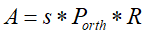
Definition A:

A = s*P.dot(R)
official

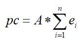
Calculate pc:

The pc calculation here is equivalent to the following formula
official

Convert the expression principal component expPC to a new matrix pc_3d of (29, 68, 3)
pc_3d = np.resize(expPC.T, [dof, n, 3])

Notice:The expPC here has been
expPC = model['expPC'][valid_ind, :n_ep]
calculated and only contains the expression principal components of the feature points. The format is (68*3,29)

Convert pc_3d to (29*68,3) format:
pc_3d = np.reshape(pc_3d, [dof*n, 3])

Calculate $pc_{2d}$ = $pc_{3d}\cdot A^T$ , pc_2d format is (29*68, 2):
pc_2d = pc_3d.dot(A.T)

Get pc after expanding pc_2d:
pc = np.reshape(pc_2d, [dof, -1]).T

define b

The formula for b is as follows:
official

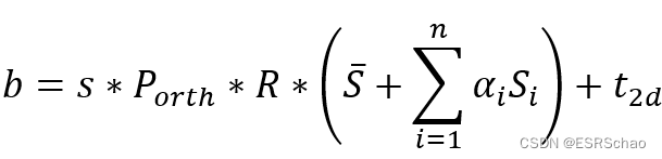
Due to the format of the matrix, some transformations must be performed first during calculation:
the shapeMU here also contains only 68 feature points.
Convert the shapeMU in the format (68*3,1) to the format (3, 68):
mu_3d = np.resize(shapeMU, [n, 3]).T
here shape = shapePC.dot(sp), that is, $\sum\limits_{i=1}^ma_iS_i$ ：
shape_3d = shape

At this point, b can be calculated according to the formula, and the obtained b format is (2,68)
b = A.dot(mu_3d + shape_3d) + np.tile(t2d[:, np.newaxis], [1, n])
and then b is converted to the format (68*2,1)
b = np.reshape(b.T, [-1, 1])

Find $\beta$

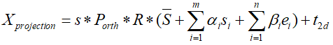
After completing the definition and calculation of A, pc and b, $X_{projection}$ The formula can be written as:
official

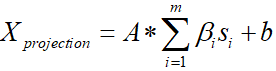
The formula put into pc can be written as:
official

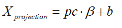
将 $X_{projection}$ The formula for is plugged into the energy equation:
official

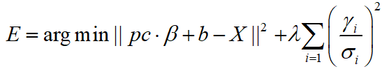
get

For $\beta$ is derived, and when the derivative is zero, $\beta$ .
The L2 norm derivation can use the formula:
official

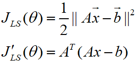
get
official

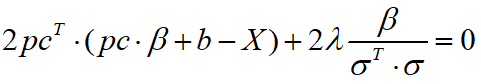
Simplify to get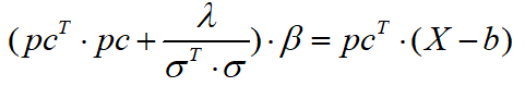 official

Then is to find $\beta$ 's code:

equation_left = np.dot(pc.T, pc) + lamb * np.diagflat(1/sigma**2)
x = np.reshape(x.T, [-1, 1])
equation_right = np.dot(pc.T, x - b)
exp_para = np.dot(np.linalg.inv(equation_left), equation_right)

$\alpha$ obtained in (2) and (3) $α$ is substituted into the energy equation, and the solution is $\alpha$

Similarly, find $\alpha$ is as follows:

expression = expPC.dot(ep)
expression = np.reshape(expression, [int(len(expression)/3), 3]).T
sp = estimate_shape(x, shapeMU, shapePC, model['shapeEV'][:n_sp,:], expression, s, R, t[:2], lamb = 0.004)

Algorithm process and finding $\beta$ $\beta$ brought in $β$ is the new value after the above calculation.

(5) Update $\alpha, \beta$ , repeat (2)-(4) for iterative update.

At this point, the code of the loop iteration part comes to an end. After multiple iterations (the number of iterations given in the program is three times), the required sp, ep, s, R, t are obtained.

back to routine

Go back to bfm.fit and
fitted_sp, fitted_ep, s, R, t = fit.fit_points(x, X_ind, self.model, n_sp = self.n_shape_para, n_ep = self.n_exp_para, max_iter = max_iter)
continue to execute downwards:

def fit(self, x, X_ind, max_iter = 4, isShow = False):
        ''' fit 3dmm & pose parameters
        Args:
            x: (n, 2) image points
            X_ind: (n,) corresponding Model vertex indices
            max_iter: iteration
            isShow: whether to reserve middle results for show
        Returns:
            fitted_sp: (n_sp, 1). shape parameters
            fitted_ep: (n_ep, 1). exp parameters
            s, angles, t
        '''
        if isShow:
            fitted_sp, fitted_ep, s, R, t = fit.fit_points_for_show(x, X_ind, self.model, n_sp = self.n_shape_para, n_ep = self.n_exp_para, max_iter = max_iter)
            angles = np.zeros((R.shape[0], 3))
            for i in range(R.shape[0]):
                angles[i] = mesh.transform.matrix2angle(R[i])
        else:
            fitted_sp, fitted_ep, s, R, t = fit.fit_points(x, X_ind, self.model, n_sp = self.n_shape_para, n_ep = self.n_exp_para, max_iter = max_iter)
            angles = mesh.transform.matrix2angle(R)
        return fitted_sp, fitted_ep, s, angles, t

angles = mesh.transform.matrix2angle(R)
Returns fitted_sp, fitted_ep, s, angles, t after converting the rotation matrix to XYZ angles .

Go back to the 3DMM routine.
fitted_sp, fitted_ep, fitted_s, fitted_angles, fitted_t = bfm.fit(x, X_ind, max_iter = 3)
After the execution is completed, continue to execute:

x = projected_vertices[bfm.kpt_ind, :2] # 2d keypoint, which can be detected from image
X_ind = bfm.kpt_ind # index of keypoints in 3DMM. fixed.

# fit
fitted_sp, fitted_ep, fitted_s, fitted_angles, fitted_t = bfm.fit(x, X_ind, max_iter = 3)

# verify fitted parameters
fitted_vertices = bfm.generate_vertices(fitted_sp, fitted_ep)
transformed_vertices = bfm.transform(fitted_vertices, fitted_s, fitted_angles, fitted_t)

image_vertices = mesh.transform.to_image(transformed_vertices, h, w)
fitted_image = mesh.render.render_colors(image_vertices, bfm.triangles, colors, h, w)

Next is
fitted_vertices = bfm.generate_vertices(fitted_sp, fitted_ep)
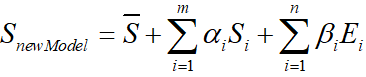
according to the calculated $\alpha ,\beta$ substitution
official

算出 $S_{newModel}$ , the corresponding source code is as follows:

 def generate_vertices(self, shape_para, exp_para):
        '''
        Args:
            shape_para: (n_shape_para, 1)
            exp_para: (n_exp_para, 1) 
        Returns:
            vertices: (nver, 3)
        '''
        vertices = self.model['shapeMU'] + \
                   self.model['shapePC'].dot(shape_para) + \
                   self.model['expPC'].dot(exp_para)
        vertices = np.reshape(vertices, [int(3), int(len(vertices)/3)], 'F').T

        return vertices

算出 $S_{newModel}$ Then perform a similar transformation on the 3D model:

transformed_vertices = bfm.transform(fitted_vertices, fitted_s, fitted_angles, fitted_t)

即 $S_{tranformed}=s\cdot R\cdot S_{newModel}+t_{3d}$

 def transform(self, vertices, s, angles, t3d):
        R = mesh.transform.angle2matrix(angles)
        return mesh.transform.similarity_transform(vertices, s, R, t3d)

Code after:

image_vertices = mesh.transform.to_image(transformed_vertices, h, w)
fitted_image = mesh.render.render_colors(image_vertices, bfm.triangles, colors, h, w)

They are converting the 3D model into a 2D image format and coloring the model with the built-in color information. I won’t explain too much here.

Result display

The generated new face image is saved to the results/3dmm directory:

# ------------- print & show 
print('pose, groudtruth: \n', s, angles[0], angles[1], angles[2], t[0], t[1])
print('pose, fitted: \n', fitted_s, fitted_angles[0], fitted_angles[1], fitted_angles[2], fitted_t[0], fitted_t[1])

save_folder = 'results/3dmm'
if not os.path.exists(save_folder):
    os.mkdir(save_folder)

io.imsave('{}/generated.jpg'.format(save_folder), image)
io.imsave('{}/fitted.jpg'.format(save_folder), fitted_image)

You can also generate a gif to show the process of feature point fitting:

# fit

fitted_sp, fitted_ep, fitted_s, fitted_angles, fitted_t = bfm.fit(x, X_ind, max_iter = 3, isShow = True)

# verify fitted parameters
for i in range(fitted_sp.shape[0]):
	fitted_vertices = bfm.generate_vertices(fitted_sp[i], fitted_ep[i])
	transformed_vertices = bfm.transform(fitted_vertices, fitted_s[i], fitted_angles[i], fitted_t[i])

	image_vertices = mesh.transform.to_image(transformed_vertices, h, w)
	fitted_image = mesh.render.render_colors(image_vertices, bfm.triangles, colors, h, w)
	io.imsave('{}/show_{:0>2d}.jpg'.format(save_folder, i), fitted_image)

options = '-delay 20 -loop 0 -layers optimize' # gif. need ImageMagick.
subprocess.call('convert {} {}/show_*.jpg {}'.format(options, save_folder, save_folder + '/3dmm.gif'), shell=True)
subprocess.call('rm {}/show_*.jpg'.format(save_folder), shell=True)

Here is the result display:

generated.jpg
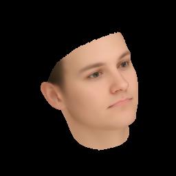
fitted.jpg

result

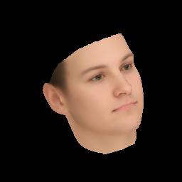
3dmm.gif

result
Of course, the new random model generated by the program will look different each time it is executed.

epilogue

After nearly a week, I finally analyzed the 3DMM routine part from beginning to end. I have learned a lot and have a lot of doubts. I will continue to update and improve these articles in the future, and I look forward to your attention.