Chapter 1, Gradient Descent and Univariate Linear Regression for Introduction to AI Artificial Intelligence (2)
Table of contents
Second, the application of linear regression
3. The general form of linear regression
4. Derivation process of unary linear regression function
Univariate linear regression on ads and cars:
The same is true about height and weight (the principle is the same as the previous one):
6. Overfitting and underfitting problems
1. What is linear regression?
Linear regression is a statistical analysis method that uses regression analysis in mathematical statistics to determine the quantitative relationship between two or more variables that depend on each other. It is widely used.
In statistics, linear regression is a type of regression analysis that models the relationship between one or more independent variables and a dependent variable using the least squares function known as the linear regression equation . Such functions are linear combinations of one or more model parameters called regression coefficients. The case of only one independent variable is called simple regression (unary regression) , and the case of more than one independent variable is called multiple regression .
Linear regression was the first type of regression analysis to be rigorously studied and widely used in practical applications. This is because models that depend linearly on their unknown parameters are easier to fit than models that depend nonlinearly on their unknown parameters, and the statistical properties of the resulting estimates are easier to determine.
Linear regression models are often fitted using the least squares approximation, but they may also be fitted using other methods, such as by minimizing the "fit flaw" in some other specification (such as least absolute error regression), or in bridge Penalty for minimizing the least-squares loss function in regression. Conversely, the least-squares approximation can be used to fit models that are nonlinear. Thus, although "least squares" and "linear models" are closely related, they are Can't draw an equal sign.
Second, the application of linear regression
math
Linear regression has many practical uses. Divided into the following two categories:
-
If the goal is prediction or mapping, linear regression can be used to fit a predictive model to the observed dataset and the values of X. After such a model is completed, for a new value of X, the fitted model can be used to predict a value of y without the corresponding y being given.
-
Given a variable y and some variables X1,...,Xp that are likely to be related to y, linear regression analysis can be used to quantify the strength of the correlation between y and Xj, and evaluate Xj that is not related to y, And identify which subsets of Xj contain redundant information about y.
Trendline
A trend line represents the long-term trend of time series data. It tells us whether a particular set of data (such as GDP, oil prices, and stock prices) has grown or fallen over a period of time. Although we can roughly draw a trendline by observing the position of the data points in the coordinate system with the naked eye, a more appropriate method is to use linear regression to calculate the position and slope of the trendline.
epidemiology
Early evidence on the effect of smoking on mortality and morbidity comes from observational studies using regression analyses . To reduce spurious correlations when analyzing observed data , researchers often include some additional variables in their regression models besides the variables of most interest. For example, suppose we have a regression model in which smoking behavior is the independent variable we are most interested in and the dependent variable is the observed lifespan of smokers over several years. Researchers may have included socioeconomic status as an additional independent variable to ensure that any observed effects of smoking on lifespan were not due to differences in education or income. However, it is impossible for us to include all variables that could confound the results into the empirical analysis. For example, a gene that doesn't exist could increase a person's chances of dying and also increase their smoking. Therefore, randomized controlled trials often produce more convincing evidence of causality than can be concluded from regression analyzes using observational data . When controlled experiments are not feasible, derivatives of regression analysis, such as instrumental variable regression, can be used to attempt to estimate causality in observed data.
finance
The capital asset pricing model uses linear regression and the concept of Beta coefficient to analyze and calculate the systematic risk of investment. This is derived directly from the model's beta coefficient linking investment returns to all risky asset returns.
economics
Linear regression is a major empirical tool in economics. For example, it is used to predict consumer spending, fixed investment spending, inventory investment, purchases of a country's export products, import spending, requirements to hold liquid assets, labor demand, and labor supply.
3. The general form of linear regression
Single linear regression analysis: Y=a+bx
Multiple linear regression analysis: Y=a+b1X1+
6X2+..+bkXk
Progressive regression model: Y=a+be-ry
Quadratic curve regression model: Y=a+bX +bX2 Hyperbolic model: Y=a+fracb]
In addition to this, there are other general forms of nonlinear regression analysis, which will not be repeated here
4. Derivation process of unary linear regression function

Manual derivation by least squares method:

Construct loss function and derivation (gradient descent method):
Gradient Descent and Least Squares
Same point:
The essence and the goal are the same: both methods are classic learning algorithms, using derivation to calculate a model (function) on the premise of Godin’s known data, so that the loss function is minimized, and then estimate and predict the given new data
difference:
Loss function: Gradient descent can choose other loss functions, and least squares must be a square loss function
Implementation method: the least square method is to directly find the global minimum; and the gradient descent is an iterative method
Effect: The least square method must find the global minimum , but the calculation is cumbersome , and there may not be a solution in complex situations; the gradient descent iteration calculation is simple , but the local minimum is generally found , and the global minimum is only when the objective function is a convex function ; The convergence speed will slow down when it reaches the minimum point, and it is extremely sensitive to the selection of the initial point
5. Related code (python)
Gradient descent:
y=(x-2.5)^2-1
import numpy as np
import matplotlib.pyplot as plt
x=np.linspace(-1,6,141)
y=(x-2.5)**2-1
#每点梯度 求导
def dj(theta) :
    return 2*(theta-2.5)
#每点的Y值
def J(theta):
  try:
    return (theta-2.5)**2-1
#防止了越来越大
  except:
    return float('inf')
#梯度下降,将theta的值记录下来,定义展大送代次数和允许的最小误差
def gradient_descent(initial_theta,eta,n_iters=1e4,error=1e-8):
    theta=initial_theta
    theta_hist.append(initial_theta)
    i_iter=0
    while i_iter<n_iters:
        gradient=dj(theta)
        last_theta=theta
        theta=theta-eta*gradient
        theta_hist.append(theta)
        if abs(J(theta)-J(last_theta))<error:
            break
        i_iter+=1
                 #绘制原始曲线和梯度下降的过程
def plot_thetahist():
    plt.plot(x,J(x))
    plt.plot(np.array(theta_hist),J(np.array(theta_hist)),color='r',marker='+')
    plt.show()
#学习率,步长
eta=0.1
theta_hist=[]
gradient_descent(0,eta,n_iters=10)
plot_thetahist()
When eta=0.1

When eta=0.4

When eta=1.1

The comparison found that the larger the step size, the stronger the oscillation and the worse the effect
Univariate linear regression on ads and cars:

import numpy as np
import matplotlib.pyplot as plt


# ---------------1. 准备数据----------
data = np.array([[1, 14],
                 [3, 24],
                 [2, 18],
                 [1, 17],
                 [3, 27]])

# 提取data中的两列数据,分别作为x,y
x = data[:, 0]
y = data[:, 1]


# 用plt画出散点图
# plt.scatter(x, y)
# plt.show()

# -----------2. 定义损失函数 均方误差 ------------------
# 损失函数是系数的函数,另外还要传入数据的x,y
def compute_cost(w, b, points):
    total_cost = 0
    M = len(points)

    # 逐点计算平方损失误差,然后求平均数
    for i in range(M):
        x = points[i, 0]
        y = points[i, 1]
        total_cost += (y - w * x - b) ** 2

    return total_cost / M


# ------------3.定义算法拟合函数-----------------
# 先定义一个求均值的函数
def average(data):
    sum = 0
    num = len(data)   #返回对象的长度
    for i in range(num):
        sum += data[i]
    return sum / num


# 定义核心拟合函数
def fit(points):
    M = len(points)
    x_bar = average(points[:, 0])

    sum_yx = 0
    sum_x2 = 0
    sum_delta = 0

    for i in range(M):
        x = points[i, 0]
        y = points[i, 1]
        sum_yx += y * (x - x_bar)
        sum_x2 += x ** 2
    # 根据公式计算w
    w = sum_yx / (sum_x2 - M * (x_bar ** 2))

    for i in range(M):
        x = points[i, 0]
        y = points[i, 1]
        sum_delta += (y - w * x)
    b = sum_delta / M

    return w, b


# ------------4. 测试------------------
w, b = fit(data)

print("w is: ", w)
print("b is: ", b)

cost = compute_cost(w, b, data)

print("cost is: ", cost)

# ---------5. 画出拟合曲线------------
plt.scatter(x, y)
# 针对每一个x,计算出预测的y值
pred_y = w * x + b

plt.plot(x, pred_y, c='r')
plt.show()
operation result:


The same is true about height and weight (the principle is the same as the previous one):
# -*- coding: utf-8 -*-
"""
Created on Tue Apr  4 17:16:29 2023

@author: Lenovo
"""

import numpy as np
import matplotlib.pyplot as plt

# ---------------1. 准备数据----------
data = np.array([[160, 58],
                 [165, 63],
                 [158, 57],
                 [172, 65],
                 [159, 62],
                 [176, 66],
                 [160, 58],
                 [162, 59],
                 [171, 62]])

# 提取data中的两列数据,分别作为x,y
x = data[:, 0]
y = data[:, 1]


# 用plt画出散点图
plt.scatter(x, y)
plt.show()

# -----------2. 定义损失函数 均方误差------------------
# 损失函数是系数的函数,另外还要传入数据的x,y
def compute_cost(w, b, points):
    total_cost = 0
    M = len(points)

    # 逐点计算平方损失误差,然后求平均数
    for i in range(M):
        x = points[i, 0]
        y = points[i, 1]
        total_cost += (y - w * x - b) ** 2

    return total_cost / M


# ------------3.定义算法拟合函数-----------------
# 先定义一个求均值的函数
def average(data):
    sum = 0
    num = len(data)
    for i in range(num):
        sum += data[i]
    return sum / num


# 定义核心拟合函数
def fit(points):
    M = len(points)
    x_bar = average(points[:, 0])

    sum_yx = 0
    sum_x2 = 0
    sum_delta = 0

    for i in range(M):
        x = points[i, 0]
        y = points[i, 1]
        sum_yx += y * (x - x_bar)
        sum_x2 += x ** 2
    # 根据公式计算w
    w = sum_yx / (sum_x2 - M * (x_bar ** 2))

    for i in range(M):
        x = points[i, 0]
        y = points[i, 1]
        sum_delta += (y - w * x)
    b = sum_delta / M

    return w, b


# ------------4. 测试------------------
w, b = fit(data)

print("w is: ", w)
print("b is: ", b)

cost = compute_cost(w, b, data)

print("cost is: ", cost)

# ---------5. 画出拟合曲线------------
plt.scatter(x, y)
# 针对每一个x,计算出预测的y值
pred_y = w * x + b

plt.plot(x, pred_y, c='r')
plt.show()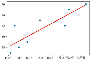
![]()
6. Overfitting and underfitting problems
Underfitting: There are many errors between the predicted value of the training set and the true value of the training set, which is called underfitting.
Overfitting: The predicted value of the training set completely fits the real value of the training set, which is called overfitting.
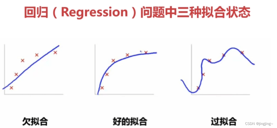


Overfitting is the training set is very good, but the test set does not work
How to avoid overfitting:
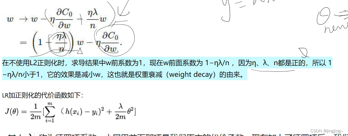
Add regular items L1, L2 (with squares, reduce high-order coefficients).

Regular term L2 derivation:


references
[EB/OL]. https://baike.baidu.com/tem/%E7%BA%BF%E6%80%A7%E5%9B%9E%E5%BD%92/8190345
[EB/OL].https://jiang-hs.gitee.io/posts/202f1f0f/,2021-3-6
[EB/OL].https://gitee.com/liyongfei_151/ml-course-share/tree/main/SimpleLinearRegression,2022-8-7
[EB/OL]. AI-4-Regression-Summary-20210128_190020_哔哩哔哩_bilibili ,2021-1-28
[EB/OL].https://blog.csdn.net/hyunbar/article/details/106294557,2020-5-22