Handwritten batch linear regression algorithm: gradient descent method implementations in Python3 model training

Author: Tarun Gupta
deephub translation Group: Meng Xiangjie

In this article, we will look to use NumPy as a program written in Python3 data processing library to learn how to implement (batch) linear regression using the gradient descent method.

I will gradually explain the working principle and the principle of each part of the code of the code.

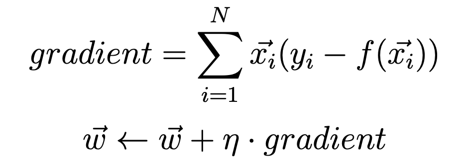
We will use this formula to calculate the gradient.

Here, x (i) is a vector of a point, where N is the size of the data set. n (eta) is our learning rate. y (i) is a target output vector. f (x) is defined as the vector f (x) = Sum (w * x) of a linear regression function, where sigma is the sum function. Further, we will consider the initial difference w0 = 0 and such that x0 = 1. All weights are initialized to 0.

In this method, we used the sum of the squared error loss function.

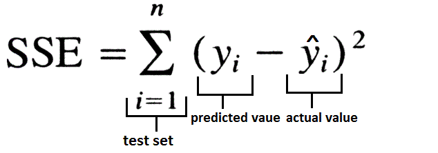
Except that SSE is initialized to zero, we will record the changes in each iteration of the SSE, and compared with a threshold value provided prior to program execution. If SSE is below the threshold, the program exits.

In this program, we provide three input from the command line. they are:

threshold - the threshold value, before the algorithm terminates, the loss must be below this threshold.
data - position data sets.
learningRate - learning rate gradient descent method.

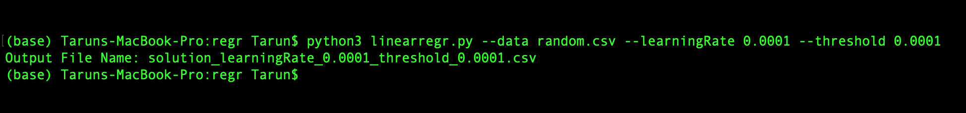
Therefore, the start of the program should look like this:

python3 linearregr.py — data random.csv — learningRate 0.0001 — threshold 0.0001

Before diving into the code we identified last thing, the program's output would be as follows:

iteration_number,weight0,weight1,weight2,...,weightN,sum_of_squared_errors

The program includes six parts, one by one we see.

Import module

import argparse # to read inputs from command line
import csv # to read the input data set file
import numpy as np # to work with the data set

Initialization part

# initialise argument parser and read arguments from command line with the respective flags and then call the main() functionif __name__ == '__main__':    
    parser = argparse.ArgumentParser()
    parser.add_argument("-d", "--data", help="Data File")
    parser.add_argument("-l", "--learningRate", help="Learning Rate")    
    parser.add_argument("-t", "--threshold", help="Threshold")    
    main()

main function part

def main():
    args = parser.parse_args()
    file, learningRate, threshold = args.data, float(
        args.learningRate), float(args.threshold) # save respective command line inputs into variables

    # read csv file and the last column is the target output and is separated from the input (X) as Y
    with open(file) as csvFile:
        reader = csv.reader(csvFile, delimiter=',')
        X = []
        Y = []
        for row in reader:
            X.append([1.0] + row[:-1])
            Y.append([row[-1]])

    # Convert data points into float and initialise weight vector with 0s.
    n = len(X)
    X = np.array(X).astype(float)
    Y = np.array(Y).astype(float)
    W = np.zeros(X.shape[1]).astype(float)
    # this matrix is transposed to match the necessary matrix dimensions for calculating dot product
    W = W.reshape(X.shape[1], 1).round(4)

    # Calculate the predicted output value
    f_x = calculatePredicatedValue(X, W)

    # Calculate the initial SSE
    sse_old = calculateSSE(Y, f_x)

    outputFile = 'solution_' + \
                 'learningRate_' + str(learningRate) + '_threshold_' \
                 + str(threshold) + '.csv'
    '''
        Output file is opened in writing mode and the data is written in the format mentioned in the post. After the
        first values are written, the gradient and updated weights are calculated using the calculateGradient function.
        An iteration variable is maintained to keep track on the number of times the batch linear regression is executed
        before it falls below the threshold value. In the infinite while loop, the predicted output value is calculated 
        again and new SSE value is calculated. If the absolute difference between the older(SSE from previous iteration) 
        and newer(SSE from current iteration) SSE is greater than the threshold value, then above process is repeated.
        The iteration is incremented by 1 and the current SSE is stored into previous SSE. If the absolute difference 
        between the older(SSE from previous iteration) and newer(SSE from current iteration) SSE falls below the 
        threshold value, the loop breaks and the last output values are written to the file.
    '''
    with open(outputFile, 'w', newline='') as csvFile:
        writer = csv.writer(csvFile, delimiter=',', quoting=csv.QUOTE_NONE, escapechar='')
        writer.writerow([*[0], *["{0:.4f}".format(val) for val in W.T[0]], *["{0:.4f}".format(sse_old)]])

        gradient, W = calculateGradient(W, X, Y, f_x, learningRate)

        iteration = 1
        while True:
            f_x = calculatePredicatedValue(X, W)
            sse_new = calculateSSE(Y, f_x)

            if abs(sse_new - sse_old) > threshold:
                writer.writerow([*[iteration], *["{0:.4f}".format(val) for val in W.T[0]], *["{0:.4f}".format(sse_new)]])
                gradient, W = calculateGradient(W, X, Y, f_x, learningRate)
                iteration += 1
                sse_old = sse_new
            else:
                break
        writer.writerow([*[iteration], *["{0:.4f}".format(val) for val in W.T[0]], *["{0:.4f}".format(sse_new)]])
    print("Output File Name: " + outputFile

Process main function is as follows:

The corresponding command line in the input to a variable
Reading the CSV file, the last one is a target output, and the input (stored as X) and stored as separate Y
Convert the data point to floating point initialization vector of weights for the 0s
Use calculatePredicatedValue function to calculate the predicted value of the output
SSE function used to calculate the initial calculateSSE
The output file is opened in write mode, data is written in the format mentioned in the article. After writing the first value, and using the gradient function calculating calculateGradient updated weight. Variable number of iterations performed to determine the linear regression performed in batch before loss function values below a threshold. While in an infinite loop, again calculated predicted output value, and calculating a new value of SSE. If the old (previous iteration from SSE) and the newer the absolute difference between (SSE from the current iteration) is greater than the threshold value, then repeat the process. Increase the number of iterations 1, SSE is currently stored in previous SSE. If the older (previous iteration of SSE) and the newer the absolute difference between the (current iteration of SSE) is below the threshold, the cycle is interrupted, and the final output value written to the file.

`calculatePredicatedValue`function

Here, the product is calculated by performing the predicted output and input matrix X W is the weight matrix points.

# dot product of X(input) and W(weights) as numpy matrices and returning the result which is the predicted output
def calculatePredicatedValue(X, W):
    f_x = np.dot(X, W)
    return f_x

`calculateGradient`function

Gradient calculated using a formula first mentioned in the article and update the weights.

def calculateGradient(W, X, Y, f_x, learningRate):
    gradient = (Y - f_x) * X
    gradient = np.sum(gradient, axis=0)
    temp = np.array(learningRate * gradient).reshape(W.shape)
    W = W + temp
    return gradient, W

`calculateSSE`function

SSE is calculated using the above equation.

def calculateSSE(Y, f_x):    
    sse = np.sum(np.square(f_x - Y))     
    return sse

Now, read the complete code. Let's look at the results of the implementation of the program.

This is like the output:

0	0.0000	0.0000	0.0000	7475.3149

1	-0.0940	-0.5376	-0.2592	2111.5105

2	-0.1789	-0.7849	-0.3766	880.6980

3	-0.2555	-0.8988	-0.4296	538.8638

4	-0.3245	-0.9514	-0.4533	399.8092

5	-0.3867	-0.9758	-0.4637	316.1682

6	-0.4426	-0.9872	-0.4682	254.5126

7	-0.4930	-0.9926	-0.4699	205.8479

8	-0.5383	-0.9952	-0.4704	166.6932

9	-0.5791	-0.9966	-0.4704	135.0293

10	-0.6158	-0.9973	-0.4702	109.3892

11	-0.6489	-0.9978	-0.4700	88.6197

12	-0.6786	-0.9981	-0.4697	71.7941

13	-0.7054	-0.9983	-0.4694	58.1631

14	-0.7295	-0.9985	-0.4691	47.1201

15	-0.7512	-0.9987	-0.4689	38.1738

16	-0.7708	-0.9988	-0.4687	30.9261

17	-0.7883	-0.9989	-0.4685	25.0544

18	-0.8042	-0.9990	-0.4683	20.2975

19	-0.8184	-0.9991	-0.4681	16.4438

20	-0.8312	-0.9992	-0.4680	13.3218

21	-0.8427	-0.9993	-0.4678	10.7925

22	-0.8531	-0.9994	-0.4677	8.7434

23	-0.8625	-0.9994	-0.4676	7.0833

24	-0.8709	-0.9995	-0.4675	5.7385

25	-0.8785	-0.9995	-0.4674	4.6490

26	-0.8853	-0.9996	-0.4674	3.7663

27	-0.8914	-0.9996	-0.4673	3.0512

28	-0.8969	-0.9997	-0.4672	2.4719

29	-0.9019	-0.9997	-0.4672	2.0026

30	-0.9064	-0.9997	-0.4671	1.6224

31	-0.9104	-0.9998	-0.4671	1.3144

32	-0.9140	-0.9998	-0.4670	1.0648

33	-0.9173	-0.9998	-0.4670	0.8626

34	-0.9202	-0.9998	-0.4670	0.6989

35	-0.9229	-0.9998	-0.4669	0.5662

36	-0.9252	-0.9999	-0.4669	0.4587

37	-0.9274	-0.9999	-0.4669	0.3716

38	-0.9293	-0.9999	-0.4669	0.3010

39	-0.9310	-0.9999	-0.4668	0.2439

40	-0.9326	-0.9999	-0.4668	0.1976

41	-0.9340	-0.9999	-0.4668	0.1601

42	-0.9353	-0.9999	-0.4668	0.1297

43	-0.9364	-0.9999	-0.4668	0.1051

44	-0.9374	-0.9999	-0.4668	0.0851

45	-0.9384	-0.9999	-0.4668	0.0690

46	-0.9392	-0.9999	-0.4668	0.0559

47	-0.9399	-1.0000	-0.4667	0.0453

48	-0.9406	-1.0000	-0.4667	0.0367

49	-0.9412	-1.0000	-0.4667	0.0297

50	-0.9418	-1.0000	-0.4667	0.0241

51	-0.9423	-1.0000	-0.4667	0.0195

52	-0.9427	-1.0000	-0.4667	0.0158

53	-0.9431	-1.0000	-0.4667	0.0128

54	-0.9434	-1.0000	-0.4667	0.0104

55	-0.9438	-1.0000	-0.4667	0.0084

56	-0.9441	-1.0000	-0.4667	0.0068

57	-0.9443	-1.0000	-0.4667	0.0055

58	-0.9446	-1.0000	-0.4667	0.0045

59	-0.9448	-1.0000	-0.4667	0.0036

60	-0.9450	-1.0000	-0.4667	0.0029

61	-0.9451	-1.0000	-0.4667	0.0024

62	-0.9453	-1.0000	-0.4667	0.0019

63	-0.9454	-1.0000	-0.4667	0.0016

64	-0.9455	-1.0000	-0.4667	0.0013

65	-0.9457	-1.0000	-0.4667	0.0010

66	-0.9458	-1.0000	-0.4667	0.0008

67	-0.9458	-1.0000	-0.4667	0.0007

68	-0.9459	-1.0000	-0.4667	0.0005

69	-0.9460	-1.0000	-0.4667	0.0004

70	-0.9461	-1.0000	-0.4667	0.0004

####最终程序

import argparse
import csv
import numpy as np


def main():
    args = parser.parse_args()
    file, learningRate, threshold = args.data, float(
        args.learningRate), float(args.threshold) # save respective command line inputs into variables

    # read csv file and the last column is the target output and is separated from the input (X) as Y
    with open(file) as csvFile:
        reader = csv.reader(csvFile, delimiter=',')
        X = []
        Y = []
        for row in reader:
            X.append([1.0] + row[:-1])
            Y.append([row[-1]])

    # Convert data points into float and initialise weight vector with 0s.
    n = len(X)
    X = np.array(X).astype(float)
    Y = np.array(Y).astype(float)
    W = np.zeros(X.shape[1]).astype(float)
    # this matrix is transposed to match the necessary matrix dimensions for calculating dot product
    W = W.reshape(X.shape[1], 1).round(4)

    # Calculate the predicted output value
    f_x = calculatePredicatedValue(X, W)

    # Calculate the initial SSE
    sse_old = calculateSSE(Y, f_x)

    outputFile = 'solution_' + \
                 'learningRate_' + str(learningRate) + '_threshold_' \
                 + str(threshold) + '.csv'
    '''
        Output file is opened in writing mode and the data is written in the format mentioned in the post. After the
        first values are written, the gradient and updated weights are calculated using the calculateGradient function.
        An iteration variable is maintained to keep track on the number of times the batch linear regression is executed
        before it falls below the threshold value. In the infinite while loop, the predicted output value is calculated 
        again and new SSE value is calculated. If the absolute difference between the older(SSE from previous iteration) 
        and newer(SSE from current iteration) SSE is greater than the threshold value, then above process is repeated.
        The iteration is incremented by 1 and the current SSE is stored into previous SSE. If the absolute difference 
        between the older(SSE from previous iteration) and newer(SSE from current iteration) SSE falls below the 
        threshold value, the loop breaks and the last output values are written to the file.
    '''
    with open(outputFile, 'w', newline='') as csvFile:
        writer = csv.writer(csvFile, delimiter=',', quoting=csv.QUOTE_NONE, escapechar='')
        writer.writerow([*[0], *["{0:.4f}".format(val) for val in W.T[0]], *["{0:.4f}".format(sse_old)]])

        gradient, W = calculateGradient(W, X, Y, f_x, learningRate)

        iteration = 1
        while True:
            f_x = calculatePredicatedValue(X, W)
            sse_new = calculateSSE(Y, f_x)

            if abs(sse_new - sse_old) > threshold:
                writer.writerow([*[iteration], *["{0:.4f}".format(val) for val in W.T[0]], *["{0:.4f}".format(sse_new)]])
                gradient, W = calculateGradient(W, X, Y, f_x, learningRate)
                iteration += 1
                sse_old = sse_new
            else:
                break
        writer.writerow([*[iteration], *["{0:.4f}".format(val) for val in W.T[0]], *["{0:.4f}".format(sse_new)]])
    print("Output File Name: " + outputFile


def calculateGradient(W, X, Y, f_x, learningRate):
    gradient = (Y - f_x) * X
    gradient = np.sum(gradient, axis=0)
    # gradient = np.array([float("{0:.4f}".format(val)) for val in gradient])
    temp = np.array(learningRate * gradient).reshape(W.shape)
    W = W + temp
    return gradient, W


def calculateSSE(Y, f_x):
    sse = np.sum(np.square(f_x - Y))

    return sse


def calculatePredicatedValue(X, W):
    f_x = np.dot(X, W)
    return f_x


if __name__ == '__main__':
    parser = argparse.ArgumentParser()
    parser.add_argument("-d", "--data", help="Data File")
    parser.add_argument("-l", "--learningRate", help="Learning Rate")
    parser.add_argument("-t", "--threshold", help="Threshold")
    main()

这篇文章介绍了使用梯度下降法进行批线性回归的数学概念。在此，考虑了损失函数（在这种情况下为平方误差总和）。我们没有看到最小化SSE的方法，而这是不应该的（需要调整学习率），我们看到了如何在阈值的帮助下使线性回归收敛。

该程序使用numpy来处理数据，也可以使用python的基础知识而不使用numpy来完成，但是它将需要嵌套循环，因此时间复杂度将增加到O（n * n）。无论如何，numpy提供的数组和矩阵的内存效率更高。另外，如果您喜欢使用pandas模块，建议您使用它，并尝试使用它来实现相同的程序。

希望您喜欢这篇文章。谢谢阅读。

原文连接：https://imba.deephub.ai/p/1b9773506e2f11ea90cd05de3860c663