foreword
Recently, I have been doing fine-tuning of the deployment of ChatGPT-like projects. I have paid more attention to two: one LLaMA and one ChatGLM. You will find that many models are fine-tuned based on these two models. When it comes to fine-tuning, how to fine-tune Well, so I took a closer look at the fine-tuning code and found that the Trainer class of the Transformers library implemented by Hugging face is generally used when fine-tuning LLM
It was found that if you want to reproduce ChatGPT from zero, you have to start from implementing Transformer, so this article is opened: How to implement Transformer, LLaMA/ChatGLM from scratch
And the biggest difference between the code interpretation of this article and other code interpretations is that each line of code that appears in this article will be commented, explained, explained, and even the variables in each line of code will be explained/explained , as always. Scholars are friendly enough so that even those without much background knowledge can understand this article smoothly
The first part implements the Transformer encoder module from scratch
How powerful is the transformer? It is basically the transformer that the infrastructure of most influential models is based on after 17 years (for example, there are more than 200 here , including but not limited to decode-based GPT, encode-based BERT, and encode-decode T5, etc.)
Through this article in the blog " Transformer Popular Notes: Gradually Understanding from Word2Vec, Seq2Seq to GPT, BERT ", we have learned the principle of transformer in detail (if you forget it, it is recommended to review it before reading this article, of course, if you are really I don’t want to jump, just want to stay in this article, that’s okay, I’ll try my best..)
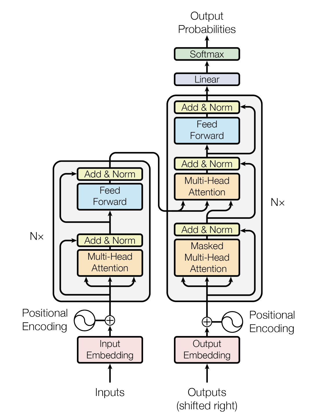
If the various details in the above picture are also displayed, it will be shown in the big picture below (this big picture comes from the source code interpretation of the Transformer model taught by Mr. Ni in July Online NLP11)
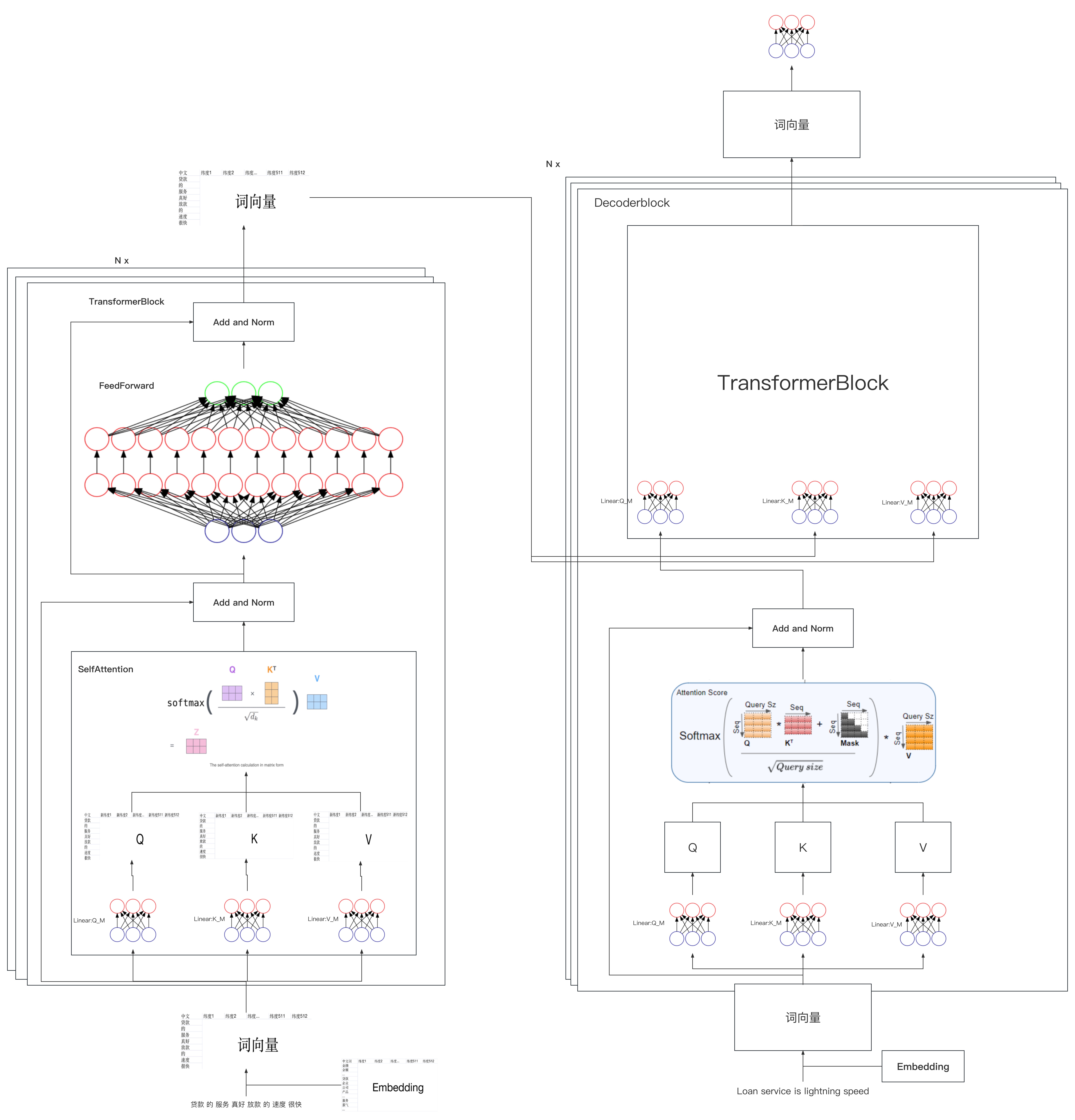
Considering that although the Transformers library implemented by Hugging face is powerful, it has more than 3,000 lines. For beginners who implement it for the first time, it is difficult to understand. Therefore, we will implement a simple version of Transformer by combining the corresponding principles step by step and coding line by line.
1.1 Processing about input: embedding for input, and then adding position encoding
In order to facilitate the writing of the following code, first introduce some libraries
import numpy as np          # 导入NumPy库,用于进行矩阵运算和数据处理
import torch                # 导入PyTorch库,用于构建神经网络及相关操作
import torch.nn as nn       # 导入PyTorch神经网络模块,用于构建神经网络层
import torch.nn.functional as F  # 导入PyTorch神经网络函数库,用于激活函数、损失函数等
import math, copy, time          # 导入数学库、复制库和时间库,用于各种数学计算、复制操作和计时
from torch.autograd import Variable  # 从PyTorch自动微分库中导入Variable类,用于构建自动微分计算图
import matplotlib.pyplot as plt      # 导入Matplotlib的pyplot模块,用于绘制图表和可视化
import seaborn  # 导入Seaborn库,用于绘制统计图形和美化图表
seaborn.set_context(context="talk")  # 设置Seaborn的上下文环境,设置图表的尺寸和标签字体大小等
%matplotlib inline                   # IPython魔术命令,使Matplotlib绘制的图形直接显示在Notebook内
1.1.1 Embedding for input
For the model, every sentence such as "The service in July is really good, and the answering speed is very fast" is a word vector in the model, but if every sentence is temporarily cramped to generate the corresponding word vector, then processing It will undoubtedly take time and effort, so in practical applications, we will pre-train various embedding matrices, these embedding matrices contain vectorized representations of commonly used words in common fields, and do word segmentation in advance
| educate | Dimension 1 | Dimension 2 | Dimension 3 | Dimension 4 | ... | Dimension 512 |
| mechanism | ||||||
| online | ||||||
| course | ||||||
| .. | ||||||
| Serve | ||||||
| answer questions | ||||||
| teacher | ||||||
| .. |
Therefore, when the model receives the input of "the service in July is really good, and the answering speed is very fast", it can search the corresponding word vector from the corresponding embedding matrix, and finally convert the entire sentence input into the corresponding vector representation
1.1.2 The deep meaning of position coding: how to code better
However, as mentioned in this article, the structure of RNN contains the timing information of the sequence, but Transformer completely loses the timing information, such as "he owes me 1 million", and "I owe him 1 million", the difference between the two The meanings are very different, so in order to solve the timing problem, the author of Transformer used a wonderful method: positional encoding (Positional Encoding).
That is, each position is numbered, so that each number corresponds to a vector. Finally, by combining the position vector and word vector as input embedding, a certain position information is introduced into each word, so that Attention can distinguish words in different positions. Yes, how to do it?
- If it is simple and rude, directly assign a number to each vector, such as between 1 and 1000
- You can also use one-hot encoding to represent the position
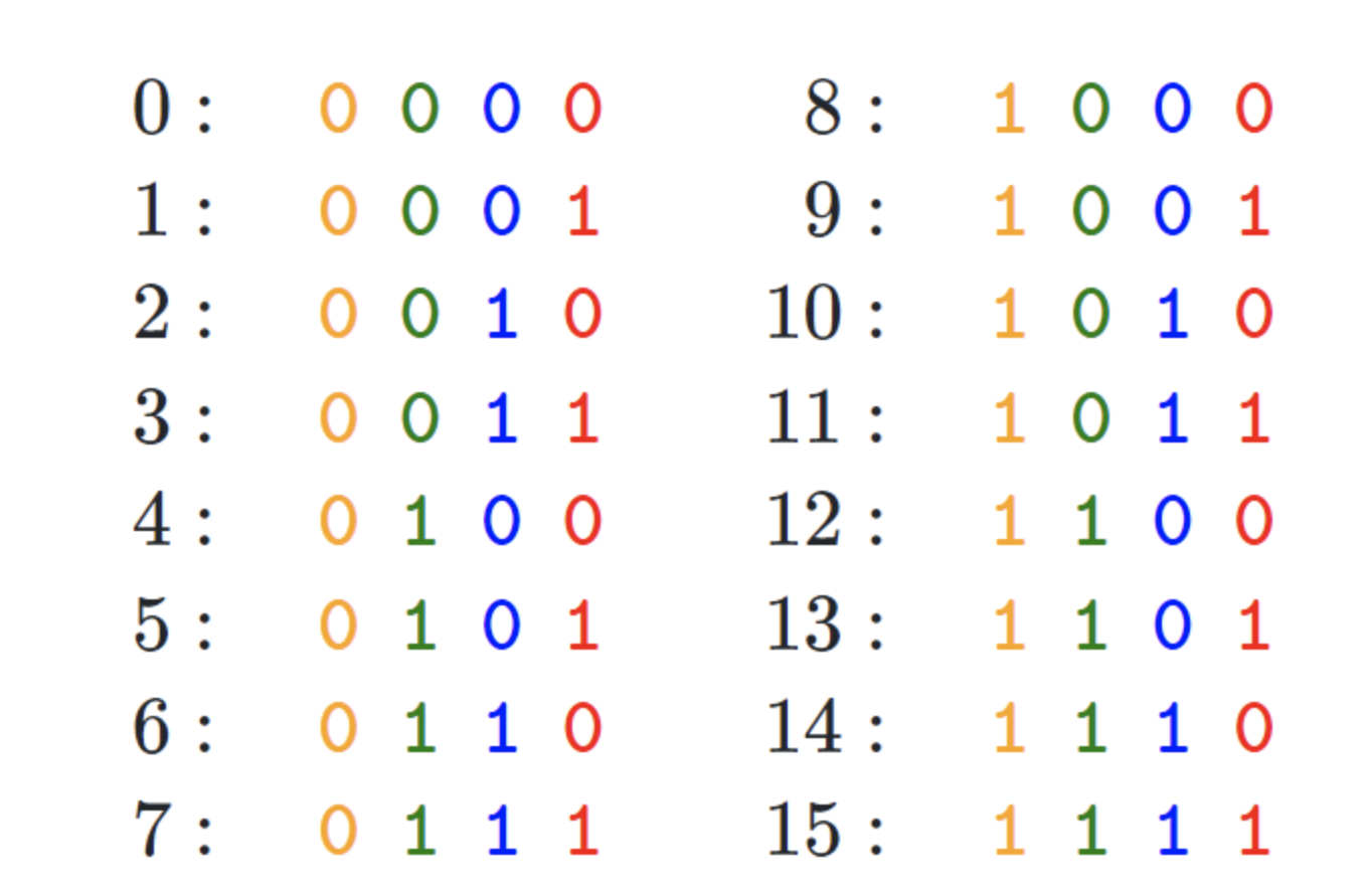
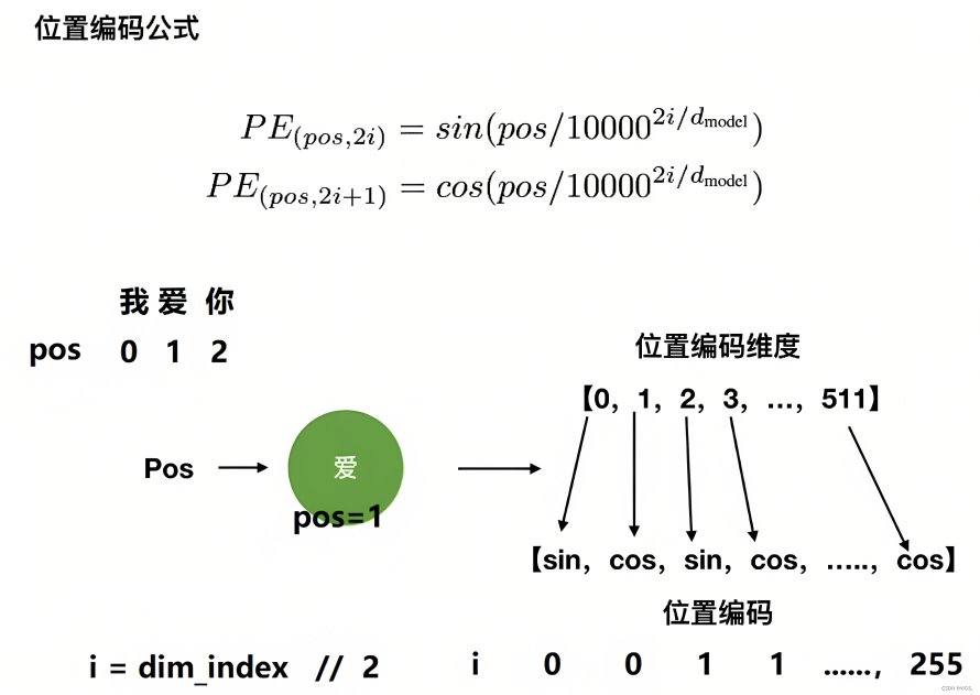
- In the transformer paper, the author creates positional encoding by alternating sin function and cos function. The formula for calculating positional encoding is as follows
Among them, pos is equivalent to the position of each token in the entire sequence, which is equivalent to 0, 1, 2, 3... (see how long the sequence is, such as 10, such as 100), and represents the dimension of the position vector (also the wordembedding The dimension, the 512 dimensions set in the transformer paper)
As
It is equivalentfor the position subscript of the embedding vector, find the quotient of 2 and round it up (double slashes can be used to
indicate integer division, that is, find the quotient and round it up), its value range is
, for example
,
,
,
,
,
,
...,
,
to the even-numbered dimension in the vector dimension, that is, the 0th dimension, the 2nd dimension, the 4th dimension..., the 510th dimension, and the sin function calculation
is the odd-numbered dimension in the vector dimension, that is, the 1st dimension, the 3rd dimension dimension, the 5th dimension.., the 511th dimension, calculated with the cos function
Don't underestimate the position code of transformer. Many people who have been doing NLP for many years may not know how in-depth the details. Most articles on the Internet talk about this position code in the same general way, and there are few In-depth, so this article will discuss in detail
Considering that a picture is worth a thousand words and an example is worth ten thousand words, for example, when we want to encode the position vector of "I love you", assuming that each token has 512 dimensions, if the position subscript starts from 0, then encode according to the position The calculation formula of can be obtained " and in order to make it clear for every reader when reading this article, I calculated the position code examples corresponding to each word (before this, these examples were basically absent elsewhere) "
- When
encoding the position of the word "I" above, its own dimension has 512 dimensions
- When
positionally encoding the word "love" above, it itself has a dimension of 512
Then superimposed on the embedding vector, we can get

- When
encoding the position of the word "you" above, its own dimension has 512 dimensions
- ....
The final visualization effect is shown in the figure below

The code is implemented as follows
‘’‘位置编码的实现,调用父类nn.Module的构造函数’‘’
class PositionalEncoding(nn.Module):
    def __init__(self, d_model, dropout, max_len=5000):
        super(PositionalEncoding, self).__init__()
        self.dropout = nn.Dropout(p=dropout)  # 初始化dropout层

        # 计算位置编码并将其存储在pe张量中
        pe = torch.zeros(max_len, d_model)  # 创建一个max_len x d_model的全零张量
        position = torch.arange(0, max_len).unsqueeze(1)  # 生成0到max_len-1的整数序列,并添加一个维度
        # 计算div_term,用于缩放不同位置的正弦和余弦函数
        div_term = torch.exp(torch.arange(0, d_model, 2) *
                             -(math.log(10000.0) / d_model))

        # 使用正弦和余弦函数生成位置编码。对于d_model的偶数索引,使用正弦函数;对于奇数索引,使用余弦函数。
        pe[:, 0::2] = torch.sin(position * div_term)
        pe[:, 1::2] = torch.cos(position * div_term)
        pe = pe.unsqueeze(0)  # 在第一个维度添加一个维度,以便进行批处理
        self.register_buffer('pe', pe)  # 将位置编码张量注册为缓冲区,以便在不同设备之间传输模型时保持其状态

    # 定义前向传播函数
    def forward(self, x):
        # 将输入x与对应的位置编码相加
        x = x + Variable(self.pe[:, :x.size(1)],
                         requires_grad=False)
        # 应用dropout层并返回结果
        return self.dropout(x)
1.2 After "embedding + position encoding", multiply by three weight matrices to get three vectors QKV
As can be seen from the figure below, the input obtained through "embedding + position encoding" will be multiplied by "three weight matrices:
" to obtain the query vector q , key vector k , and value vector v (you can simply and rudely understand it as three weight matrices: avatars), and then perform a down-linear transformation
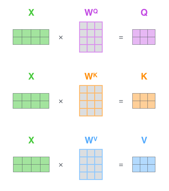
To do this, we can first create four identical linear layers, each with an input dimension of d_model and an output dimension of d_model
self.linears = clones(nn.Linear(d_model, d_model), 4) The first three linear layers are used to linearly transform the q vector, k vector, and v vector respectively (as for the fourth linear layer in the subsequent third point)
1.3 Do Add&Norm on the input and Multi-Head Attention, and then do Add&Norm on the output of the previous step and Feed Forward
Let's focus on this part of the original image in the transformer paper. It can be seen that after the input is encoded by embedding+position, first do the following two steps
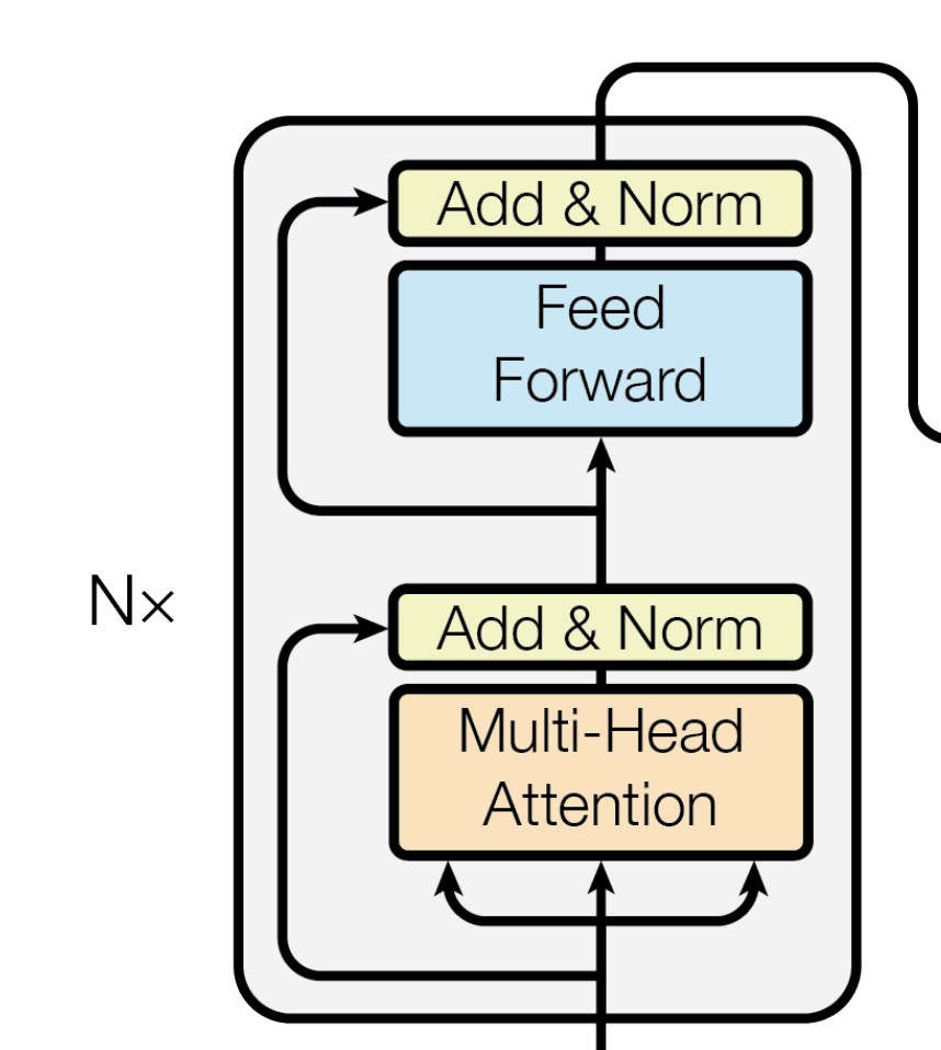
- Do multi-head attention for the query vector, and add and normalize the obtained result to the original query vector
What kind of addition method is this addition? In fact, the Residual Connection (residual connection) represented by Add is to solve the difficult problem of multi-layer neural network training. By passing the information of the previous layer to the next layer without difference, it can effectively only focus on the difference. This method was often used in image processing structures such as ResNet beforeattention = self.attention(query, key, value, mask) output = self.dropout(self.norm1(attention + query))
This function is realized through the SublayerConnection function during specific coding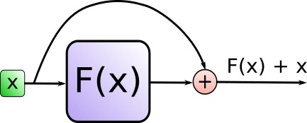
Norm represents Layer Normalization. By normalizing the activation value of the layer, the training process of the model can be accelerated to make it converge faster. The LayerNorm function is used to realize the encoding ."""一个残差连接(residual connection),后面跟着一个层归一化(layer normalization)操作""" class SublayerConnection(nn.Module): # 初始化函数,接收size(层的维度大小)和dropout(dropout率)作为输入参数 def __init__(self, size, dropout): super(SublayerConnection, self).__init__() # 调用父类nn.Module的构造函数 self.norm = LayerNorm(size) # 定义一个层归一化(Layer Normalization)操作,使用size作为输入维度 self.dropout = nn.Dropout(dropout) # 定义一个dropout层 # 定义前向传播函数,输入参数x是输入张量,sublayer是待执行的子层操作 def forward(self, x, sublayer): # 将残差连接应用于任何具有相同大小的子层 # 首先对输入x进行层归一化,然后执行子层操作(如self-attention或前馈神经网络) # 接着应用dropout,最后将结果与原始输入x相加。 return x + self.dropout(sublayer(self.norm(x)))'''构建一个层归一化(layernorm)模块''' class LayerNorm(nn.Module): # 初始化函数,接收features(特征维度大小)和eps(防止除以零的微小值)作为输入参数 def __init__(self, features, eps=1e-6): super(LayerNorm, self).__init__() # 调用父类nn.Module的构造函数 self.a_2 = nn.Parameter(torch.ones(features)) # 定义一个大小为features的一维张量,初始化为全1,并将其设置为可训练参数 self.b_2 = nn.Parameter(torch.zeros(features)) # 定义一个大小为features的一维张量,初始化为全0,并将其设置为可训练参数 self.eps = eps # 将防止除以零的微小值eps保存为类实例的属性 # 定义前向传播函数,输入参数x是输入张量 def forward(self, x): mean = x.mean(-1, keepdim=True) # 计算输入x在最后一个维度上的均值,保持输出结果的维度 std = x.std(-1, keepdim=True) # 计算输入x在最后一个维度上的标准差,保持输出结果的维度 # 对输入x进行层归一化,使用可训练参数a_2和b_2进行缩放和偏移,最后返回归一化后的结果 return self.a_2 * (x - mean) / (std + self.eps) + self.b_2 - After the "output result output of the above step is used as feed forward", it is added to the "original output result output of the above step" and normalized
        forward = self.feed_forward(output)
        block_output = self.dropout(self.norm2(forward + output))
        return block_output
This encoder layer code can be fully written as
"""编码器(Encoder)由自注意力(self-attention)层和前馈神经网络(feed forward)层组成"""
class EncoderLayer(nn.Module):
    # 初始化函数,接收size(层的维度大小)、self_attn(自注意力层实例)、feed_forward(前馈神经网络实例)和dropout(dropout率)作为输入参数
    def __init__(self, size, self_attn, feed_forward, dropout):
        super(EncoderLayer, self).__init__()      # 调用父类nn.Module的构造函数
        self.self_attn = self_attn                # 将自注意力层实例保存为类实例的属性
        self.feed_forward = feed_forward          # 将前馈神经网络实例保存为类实例的属性
        self.sublayer = clones(SublayerConnection(size, dropout), 2)  # 创建两个具有相同参数的SublayerConnection实例(用于残差连接和层归一化)
        self.size = size                          # 将层的维度大小保存为类实例的属性

    # 先对输入x进行自注意力操作,然后将结果传递给第一个SublayerConnection实例(包括残差连接和层归一化)
    def forward(self, x, mask):
        x = self.sublayer[0](x, lambda x: self.self_attn(x, x, x, mask))
        # 将上一步的输出传递给前馈神经网络,然后将结果传递给第二个SublayerConnection实例(包括残差连接和层归一化),最后返回结果
        return self.sublayer[1](x, self.feed_forward)
1.3.1 Scaled Dot-Product Attention
Next, let's look at the overall implementation steps of Scaled Dot-Product Attention
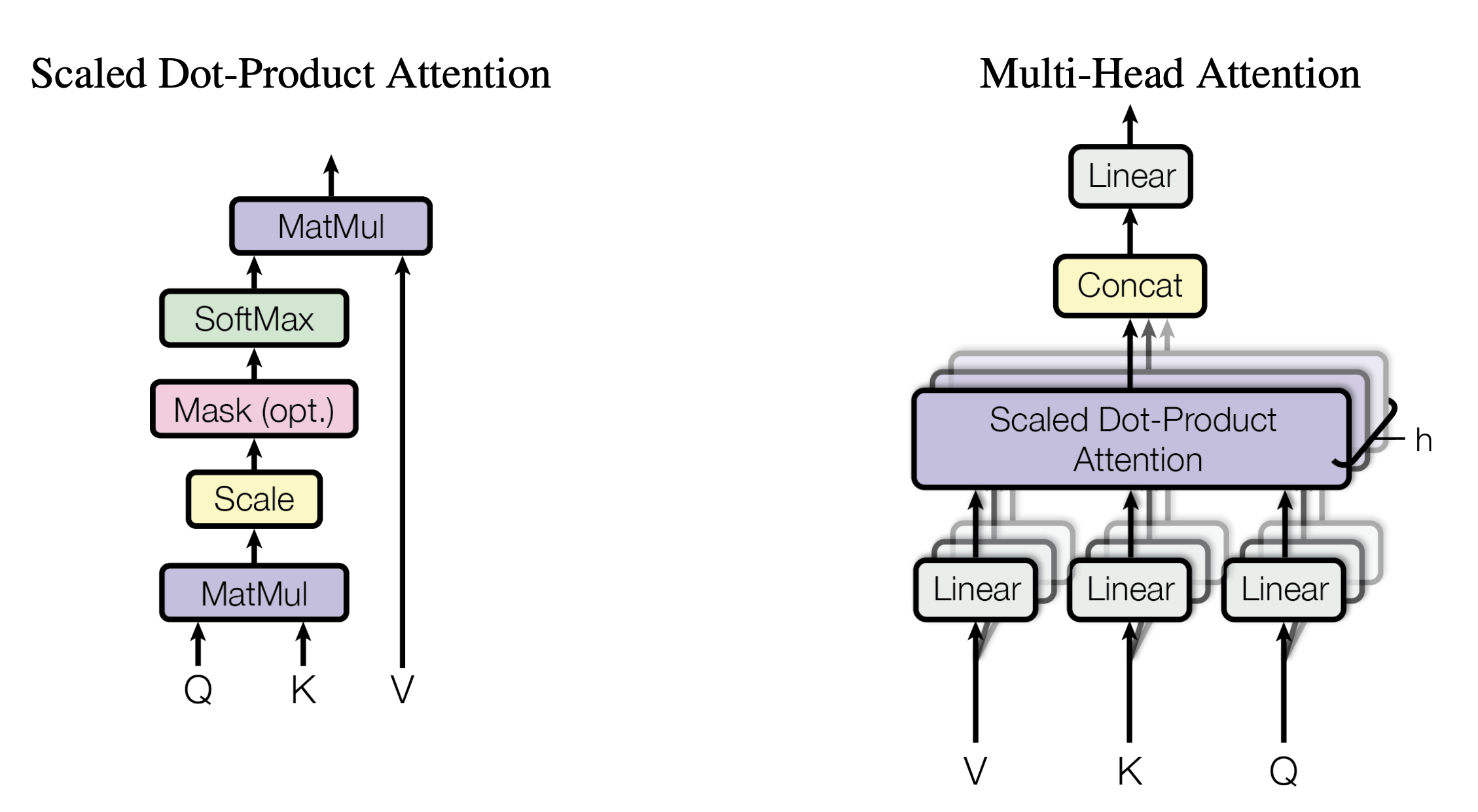
- In order to calculate the similarity between each word and other words, the dot product of " the q vector of each word/token " and " the k vector of all words/token including itself " will be done one by one (the difference between the two vectors The dot product result between can represent the similarity of two vectors)
Corresponding to the form of the matrix, the matrix Q is multiplied by the transpose of the K matrix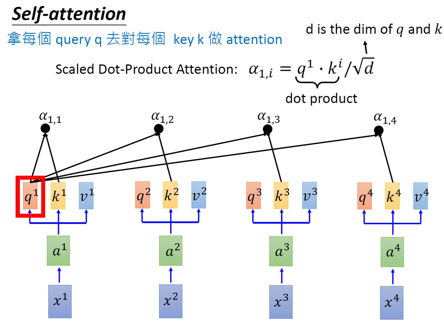
. For example, suppose the word in a sentence is: 1 2 3 4, then the transpose of Q multiplied by K isshown in the figure below
The final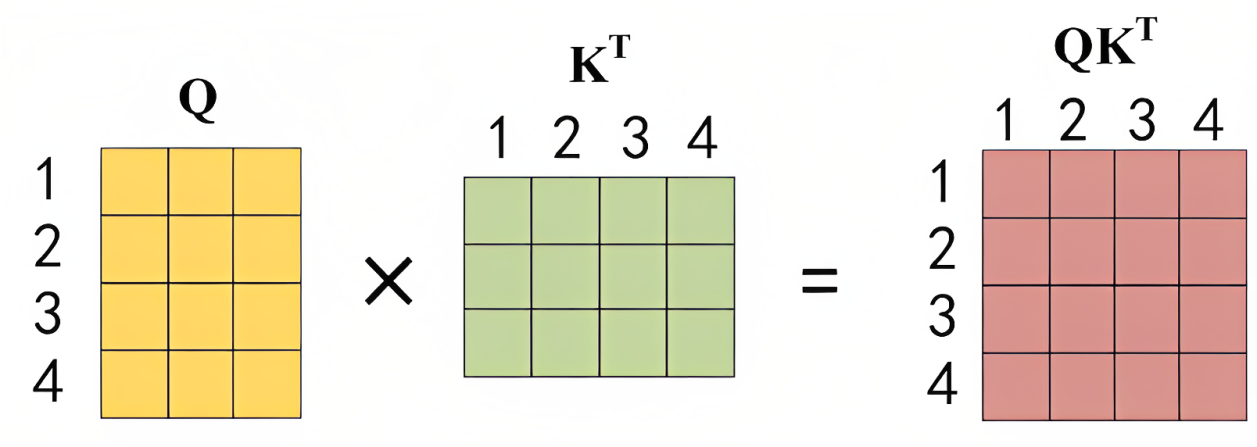
matrix has 4 rows and 4 columns. If you look at it row by row from top to bottom, there will be a value in each grid, and each value represents in turn: the dot product
results or similarity of words 1 and 1 2 3 4 , for example, it may be 0.5 0.2 0.2 0.1, which represents the amount of attention placed on 1 2 3 4 when encoding 1 At the same
time, it can be seen that when the model encodes the information of the current position, it will excessively focus on its own Position (of course, this is understandable, after all, I am the most similar to myself), but may ignore other positions. You will soon see that one solution the author adopts is to use Multi-Head Attention (Multi-Head Attention) - Since
it will increase as the dimension increases, in order to avoid being too large, dividing by
is equivalent to scaling down the result of the dot product
Among them,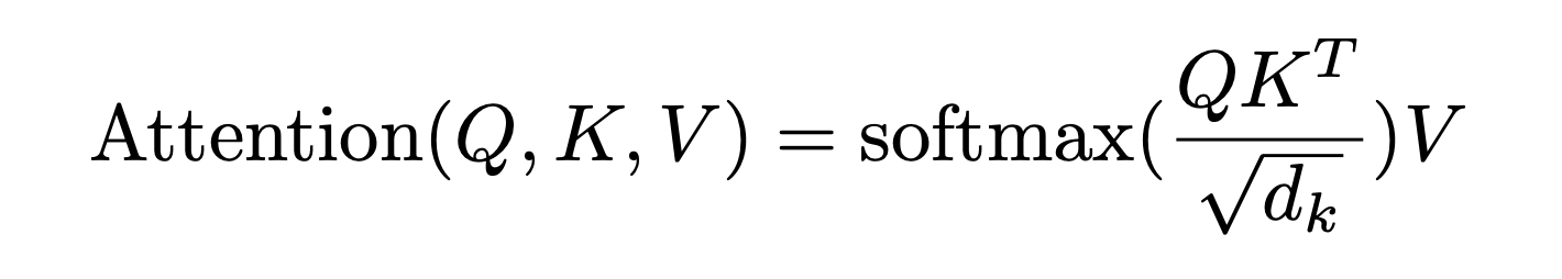
is the dimension of the vector
, and
if only one head is set, it
, and the dimension of the model is 512 dimensions, then it
The code of the above two steps can be written as follows# torch.matmul是PyTorch库提供的矩阵乘法函数 # 具体操作即是将第一个矩阵的每一行与第二个矩阵的每一列进行点积(对应元素相乘并求和),得到新矩阵的每个元素 scores = torch.matmul(query, key.transpose(-2, -1)) \ / math.sqrt(d_k) - Then use Softmax to calculate the Attention value of each word for other words, and the sum of these values is 1 (equivalent to a normalized effect)
The code corresponding to this step is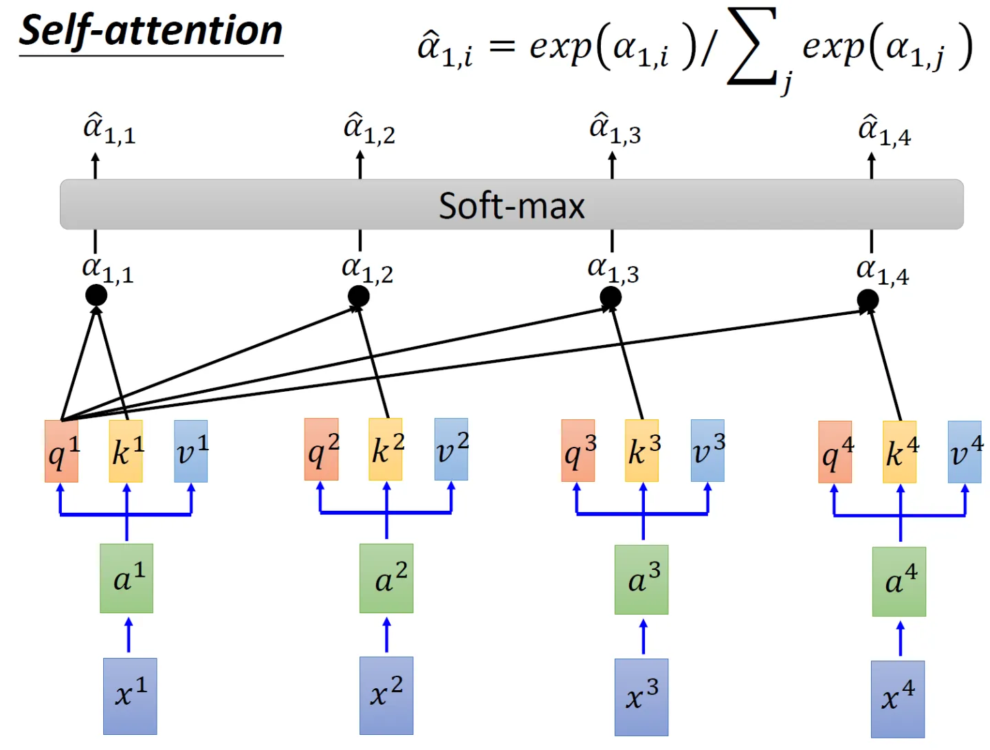
# 对 scores 进行 softmax 操作,得到注意力权重 p_attn p_attn = F.softmax(scores, dim = -1) - Finally, multiply by
the matrix, that is, for all values (v1 v2 v3 v4), according to different attention values (
), do a weighted average
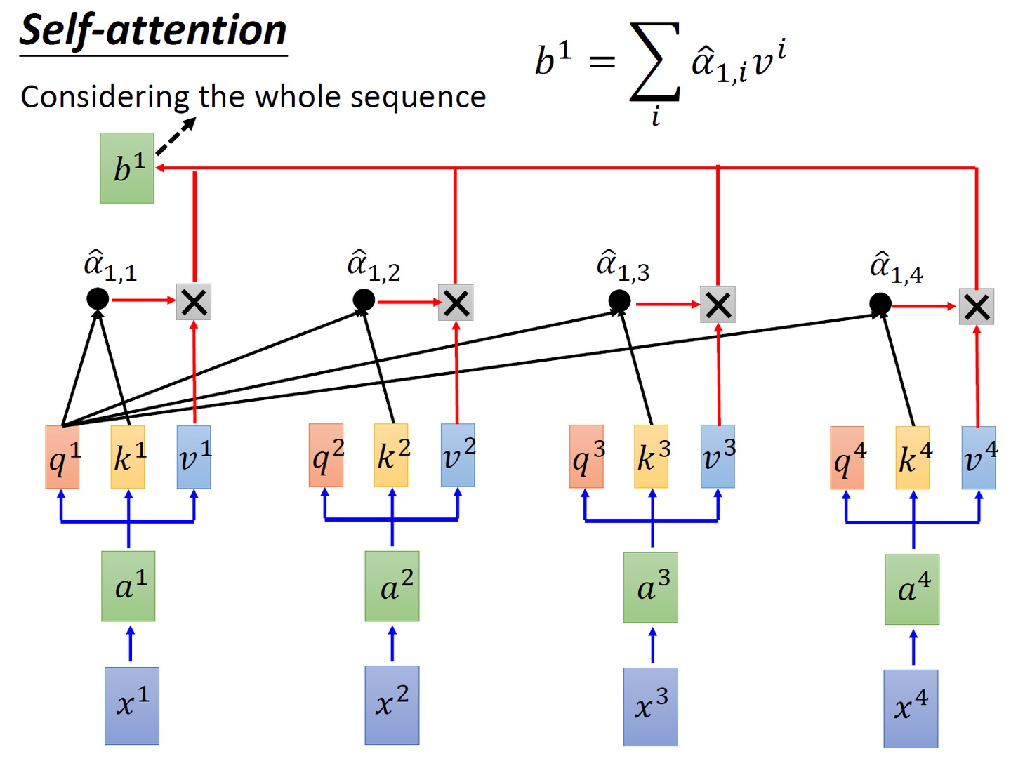
- Finally, the output of the word is obtained, as shown in the figure below (the 4 rows of the V matrix in the figure represent v1 v2 v3 v4 respectively):
The code corresponding to the above two steps is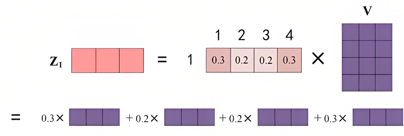
    # 用注意力权重 p_attn 对 value 向量进行加权求和,得到最终的输出
    return torch.matmul(p_attn, value), p_attn
Finally, the complete code corresponding to this part of Scaled Dot-Product Attention can be written as
'''计算“缩放点积注意力'''
# query, key, value 是输入的向量组
# mask 用于遮掩某些位置,防止计算注意力
# dropout 用于添加随机性,有助于防止过拟合
def attention(query, key, value, mask=None, dropout=None):

    d_k = query.size(-1)  # 获取 query 向量的最后一个维度的大小,即词嵌入的维度

    # 计算 query 和 key 的点积,并对结果进行缩放,以减少梯度消失或爆炸的可能性
    scores = torch.matmul(query, key.transpose(-2, -1)) \
             / math.sqrt(d_k)

    # 如果提供了 mask,根据 mask 对 scores 进行遮掩
    # 遮掩的具体方法就是设为一个很大的负数比如-1e9,从而softmax后 对应概率基本为0
    if mask is not None:
        scores = scores.masked_fill(mask == 0, -1e9)

    # 对 scores 进行 softmax 操作,得到注意力权重 p_attn
    p_attn = F.softmax(scores, dim = -1)

    # 如果提供了 dropout,对注意力权重 p_attn 进行 dropout 操作
    if dropout is not None:
        p_attn = dropout(p_attn)

    # 用注意力权重 p_attn 对 value 向量进行加权求和,得到最终的输出
    return torch.matmul(p_attn, value), p_attn
1.3.2 Multi-Head Attention
Let’s look at the example of 2 heads first, still by generating the corresponding three matrices
,
,
, and then multiplying these three matrices by two transfer matrices to get the corresponding sub-matrix, such as
The two sub-matrices corresponding to the matrix
,
The two sub-matrices corresponding to the matrix are
,
The two sub-matrices corresponding to the matrix are
,
As for the same reason, the corresponding 6 sub-matrices are also generated
,
,
,
,
,
When coding next , in two steps
do the dot product and multiply
, and then add the results of these two calculations to get
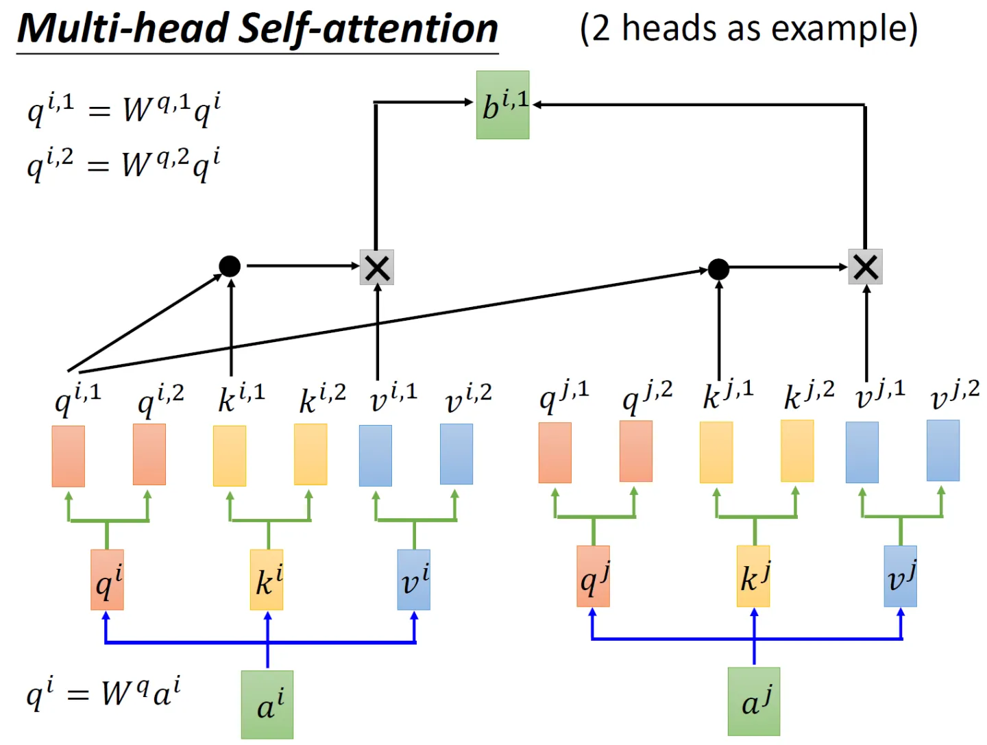
Then
do the dot product and then multiply
, then
do the dot product and then multiply
, and then add the results of these two calculations to get

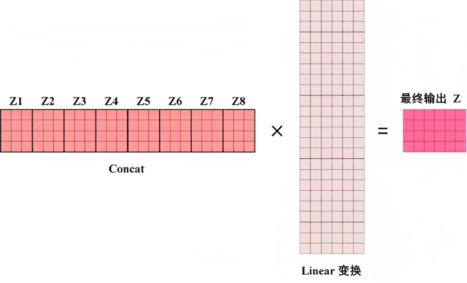
If there are 8 heads, the calculation steps are the same, just change from 2 heads to 8 heads, and finally concat the results obtained by each head directly, and finally go through a linear transformation to get the final output. The whole is as follows
This part of the Multi-Head Attention code can be written as
'''代码来自nlp.seas.harvard.edu,我针对每一行代码、甚至每行代码中的部分变量都做了详细的注释/解读'''
class MultiHeadedAttention(nn.Module):
    # 输入模型的大小(d_model)和注意力头的数量(h)
    def __init__(self, h, d_model, dropout=0.1):
        super(MultiHeadedAttention, self).__init__()
        assert d_model % h == 0  # 确保 d_model 可以被 h 整除

        # 我们假设 d_v(值向量的维度)总是等于 d_k(键向量的维度)
        self.d_k = d_model // h      # 计算每个注意力头的维度
        self.h = h                   # 保存注意力头的数量
        self.linears = clones(nn.Linear(d_model, d_model), 4)  # 上文解释过的四个线性层
        self.attn = None                      # 初始化注意力权重为 None
        self.dropout = nn.Dropout(p=dropout)  # 定义 dropout 层

    # 实现多头注意力的前向传播
    def forward(self, query, key, value, mask=None):
        if mask is not None:
            # 对所有 h 个头应用相同的 mask
            mask = mask.unsqueeze(1)
        nbatches = query.size(0)  # 获取 batch 的大小

        # 1) 批量执行从 d_model 到 h x d_k 的线性投影
        query, key, value = \
            [l(x).view(nbatches, -1, self.h, self.d_k).transpose(1, 2)
             for l, x in zip(self.linears, (query, key, value))]

        # 2) 在批量投影的向量上应用注意力
        # 具体方法是调用上面实现Scaled Dot-Product Attention的attention函数
        x, self.attn = attention(query, key, value, mask=mask,
                                 dropout=self.dropout)

        # 3) 使用 view 函数进行“拼接concat”,然后做下Linear变换
        x = x.transpose(1, 2).contiguous() \
             .view(nbatches, -1, self.h * self.d_k)
        return self.linears[-1](x)  # 返回多头注意力的输出
1.3.3 Implementation of Position-wise feedforward network
In the above, we implemented embedding, position encoding, scaling dot product/multi-head attention, and Add and Norm one by one. The last module left in the entire encoder part is the Feed Forward Network (FFN for short) in the frame below.
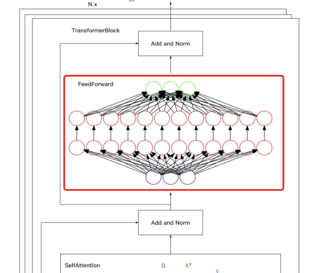
It includes two linear transformations: first expand and then shrink in dimension, the dimension of the final input and output is , the dimension of the inner layer is
, and ReLU is used as the activation function in the process
Although the linear transformations are the same at different positions, they use different parameters from layer to layer, which is equivalent to using two convolutions with kernel size 1
This part of the code can be written as follows
‘’‘定义一个名为PositionwiseFeedForward的类,继承自nn.Module’‘’
class PositionwiseFeedForward(nn.Module):
    # 文档字符串:实现FFN方程
    # 初始化方法,接受三个参数:d_model,d_ff和dropout(默认值为0.1)
    def __init__(self, d_model, d_ff, dropout=0.1):
        # 调用父类nn.Module的初始化方法
        super(PositionwiseFeedForward, self).__init__()
        self.w_1 = nn.Linear(d_model, d_ff)  # 定义一个全连接层,输入维度为d_model,输出维度为d_ff
        self.w_2 = nn.Linear(d_ff, d_model)  # 定义一个全连接层,输入维度为d_ff,输出维度为d_model
        self.dropout = nn.Dropout(dropout)  # 定义一个dropout层,dropout概率为传入的dropout参数

    # 定义前向传播方法,接受一个输入参数x
    def forward(self, x):
        # 将输入x通过第一个全连接层w_1后,经过ReLU激活函数,再通过dropout层,最后通过第二个全连接层w_2,返回最终结果
        return self.w_2(self.dropout(F.relu(self.w_1(x))))
1.4 Copy N copies of the entire transformer block and finally form the entire encode module
N can be equal to 6
class Encoder(nn.Module):  # 定义一个名为Encoder的类,它继承了nn.Module类
    # 一个具有N层堆叠的核心编码器
    # 初始化方法,接受两个参数:layer(编码器层的类型)和N(编码器层的数量)
    def __init__(self, layer, N):
        super(Encoder, self).__init__()  # 调用父类nn.Module的初始化方法
        self.layers = clones(layer, N)  # 创建N个编码器层的副本,并将其赋值给实例变量self.layers
        self.norm = LayerNorm(layer.size)  # 创建一个LayerNorm层,并将其赋值给实例变量self.norm

    # 定义前向传播方法,接受两个参数:x(输入数据)和mask(掩码)
    def forward(self, x, mask):
        # 文档字符串:解释本方法的功能是将输入(及其掩码)依次传递给每一层
        for layer in self.layers:  # 遍历self.layers中的每一个编码器层
            x = layer(x, mask)  # 将输入x和mask传递给当前编码器层,并将输出结果赋值给x
        return self.norm(x)  # 对最终的输出x应用LayerNorm层,并将结果返回
The code of the clone function is
def clones(module, N):
    "Produce N identical layers."
    return nn.ModuleList([copy.deepcopy(module) for _ in range(N)])
The second part implements the Transformer decoder module from zero
Let's review the entire model architecture of the transformer, especially the decoder part. After all, besides BERT, GPT and other influential models use the transformer decode structure.

from bottom to top,
- The input consists of 2 parts, below is the embedding of the output of the previous time step
plus a Positional Encoding representing the position - Then there is Masked Multi-Head Self-attention. Masked means that the attention will only attend on the sequence that has been generated. This is very reasonable, because the things that have not been generated do not exist, so you cannot do attention and then do Add&
Norm - Further up is a Multi-Head Attention layer without a mask. Its Key and Value matrices use the encoding information matrix of the Encoder, and the Query uses the output calculation of the previous Decoder block and then do Add&
Norm - Continue to go up, after a FFN layer, also do Add&Norm
- Finally, after doing the linear transformation, calculate the probability of the next translated word through the Softmax layer
2.1 Masked Multi-Head Self-attention
// to be updated

The third part is the code structure and implementation of LLaMA and ChatGLM-6B
// To be updated..
The fourth part how to speed up the training and tuning of the model
// This article is being updated every day. It is expected to complete the first draft by the end of April and basically take shape by the end of May..
References and Recommended Reading
- Transformer popular notes: gradually understand from Word2Vec, Seq2Seq to GPT, BERT
- Transformer original paper (worth reading several times): Attention Is All You Need
- Vision Transformer super detailed interpretation (principle analysis + code interpretation) (1)
- Detailed explanation of the Transformer model (the most complete version of the diagram)
- The Annotated Transformer ( one of the translations ), harvard's simple coding implementation of transformer
- What are the details of the transformer?
- How to understand transformer from shallow to deep?
- Transformer Architecture: The Positional Encoding | Transformer Architecture: The Positional Encoding
- Transformer study notes 1: Positional Encoding (positional encoding)
- Nanny-level explanation of Transformer
Addendum: Creation/Modification Log
- 4.12-4.14, basically completed the first draft of the transformer encoder part of the first part
- 4.16, thoroughly improve the description of transformer position encoding, it may be the most clear description of this point on the Internet