1 model of thinking
Transformer, abandoned the traditional CNN and RNN, the entire network structure composed entirely of Attention mechanism. The reason of using the mechanism Attention is given to the RNN (or LSTM, GRU, etc.) is calculated as the limit order, which means that RNN correlation algorithm can calculate from left to right or right to left calculation, this mechanism two questions arise:
Transformer is made to solve the above two issues:
2 model architecture
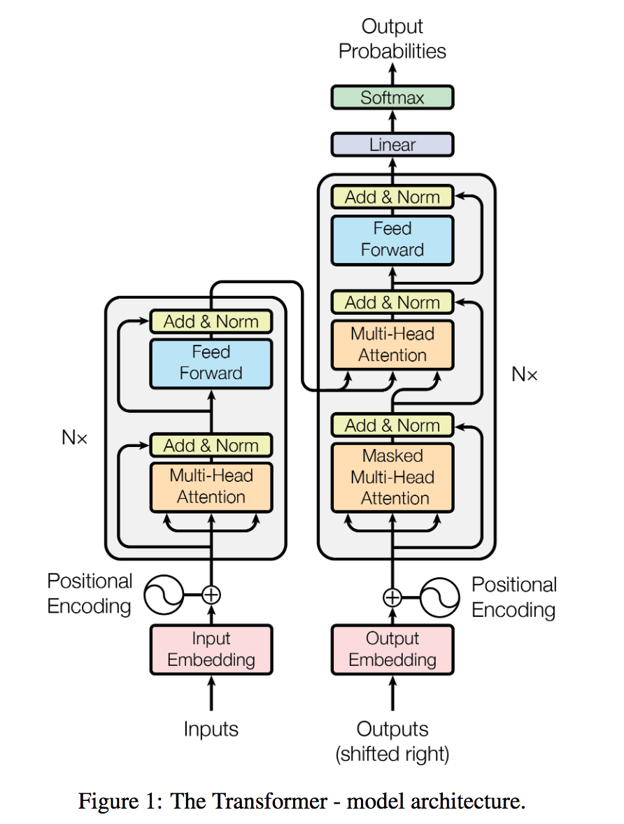
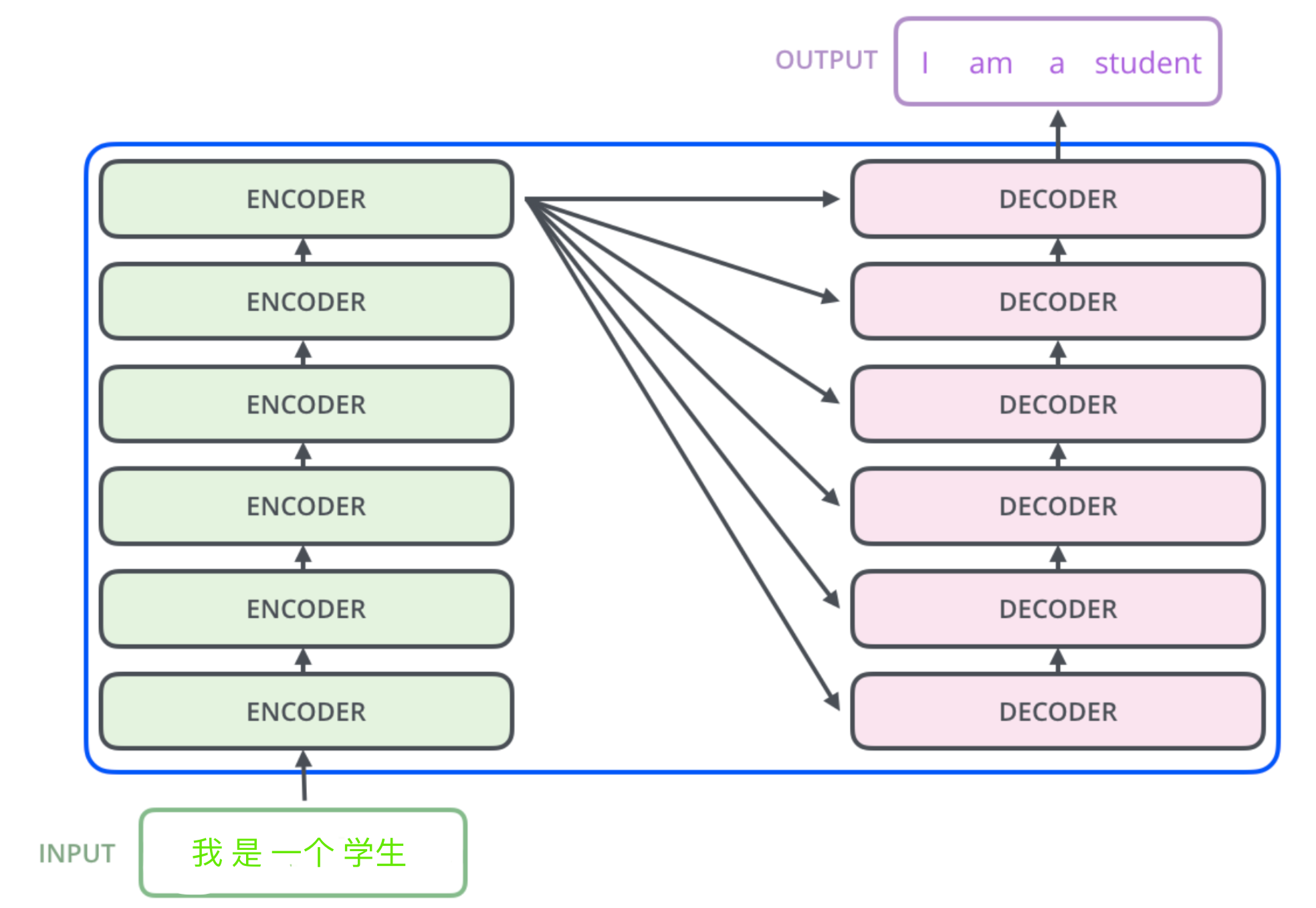
Above, a structure of the transformer Encoder-Decoder Model nature. First input sequence for Embedding, after binding Encoder output once again input Decoder, a word sequence probability calculation last softmax.
3 Embedding
is input transformer Word Embedding Embedding the Position + .
3.1 Word Embedding
class Embeddings(nn.Module):
    def __init__(self, d_model, vocab):
        super(Embeddings, self).__init__()
        self.lut = nn.Embedding(vocab, d_model)
        self.d_model = d_model  #表示embedding的维度

    def forward(self, x):
        return self.lut(x) * math.sqrt(self.d_model)
3.2 Positional Embedding
在RNN中,对句子的处理是一个个word按顺序输入的。但在 Transformer 中,输入句子的所有word是同时处理的,没有考虑词的排序和位置信息。因此,Transformer 的作者提出了加入 “positional encoding” 的方法来解决这个问题。“positional encoding“”使得 Transformer 可以衡量 word 位置有关的信息。
如何实现具有位置信息的encoding呢?作者提供了两种思路:
- 通过训练学习 positional encoding 向量;
- 使用公式来计算 positional encoding向量。
试验后发现两种选择的结果是相似的,所以采用了第2种方法,优点是不需要训练参数,而且即使在训练集中没有出现过的句子长度上也能用。
# Positional Encoding
class PositionalEncoding(nn.Module):
    "实现PE功能"
    def __init__(self, d_model, dropout, max_len=5000):
        super(PositionalEncoding, self).__init__()
        self.dropout = nn.Dropout(p=dropout)

        pe = torch.zeros(max_len, d_model)
        position = torch.arange(0., max_len).unsqueeze(1)
        div_term = torch.exp(torch.arange(0., d_model, 2) *
                             -(math.log(10000.0) / d_model))

        pe[:, 0::2] = torch.sin(position * div_term)    # 偶数列
        pe[:, 1::2] = torch.cos(position * div_term)    # 奇数列
        pe = pe.unsqueeze(0)           # [1, max_len, d_model]
        self.register_buffer('pe', pe)

    def forward(self, x):
        x = x + Variable(self.pe[:, :x.size(1)], requires_grad=False)
        return self.dropout(x)
# 在位置编码下方,将基于位置添加正弦波。对于每个维度,波的频率和偏移都不同。
plt.figure(figsize=(15, 5))
pe = PositionalEncoding(20, 0)
y = pe.forward(Variable(torch.zeros(1, 100, 20)))
plt.plot(np.arange(100), y[0, :, 4:8].data.numpy())
plt.legend(["dim %d"%p for p in [4,5,6,7]])
输出图像:
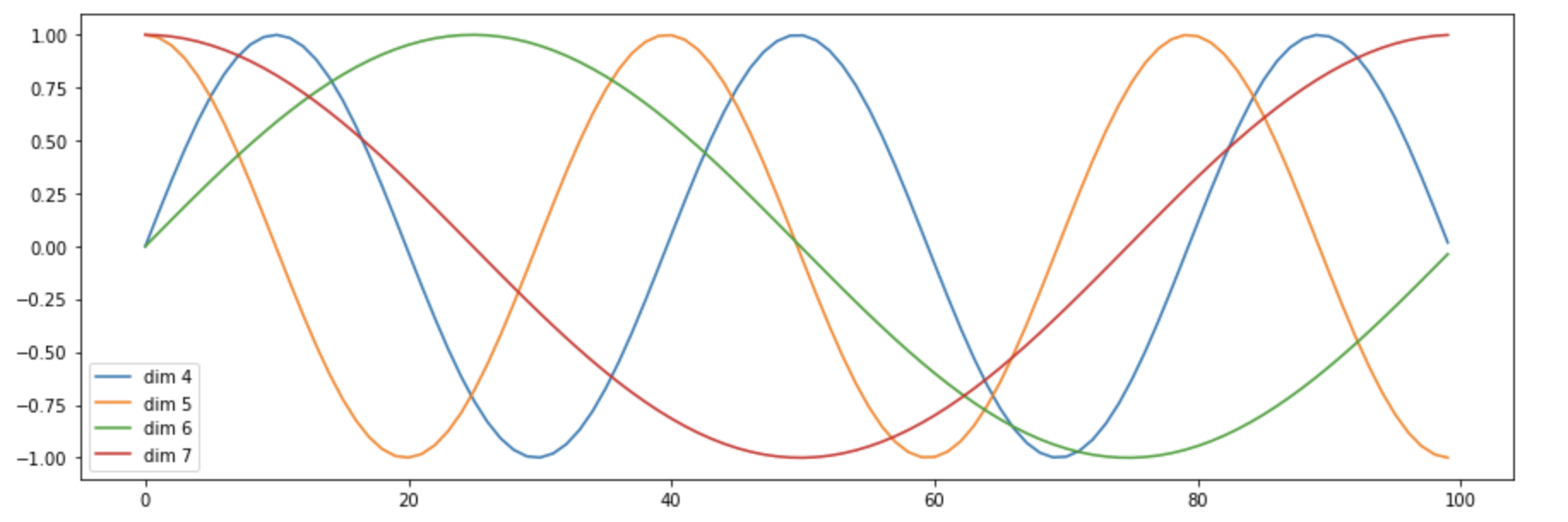
可以看到某个序列中不同位置的单词,在某一维度上的位置编码数值不一样,即同一序列的不同单词在单个纬度符合某个正弦或者余弦,可认为他们的具有相对关系。
4 Encoder
4.1 Muti-Head-Attention
4.1.1 Self-Attention
key(K), x经过第三个线性变换得到value(V)。
- key = linear_k(x)
- query = linear_q(x)
- value = linear_v(x)
用矩阵表示即:
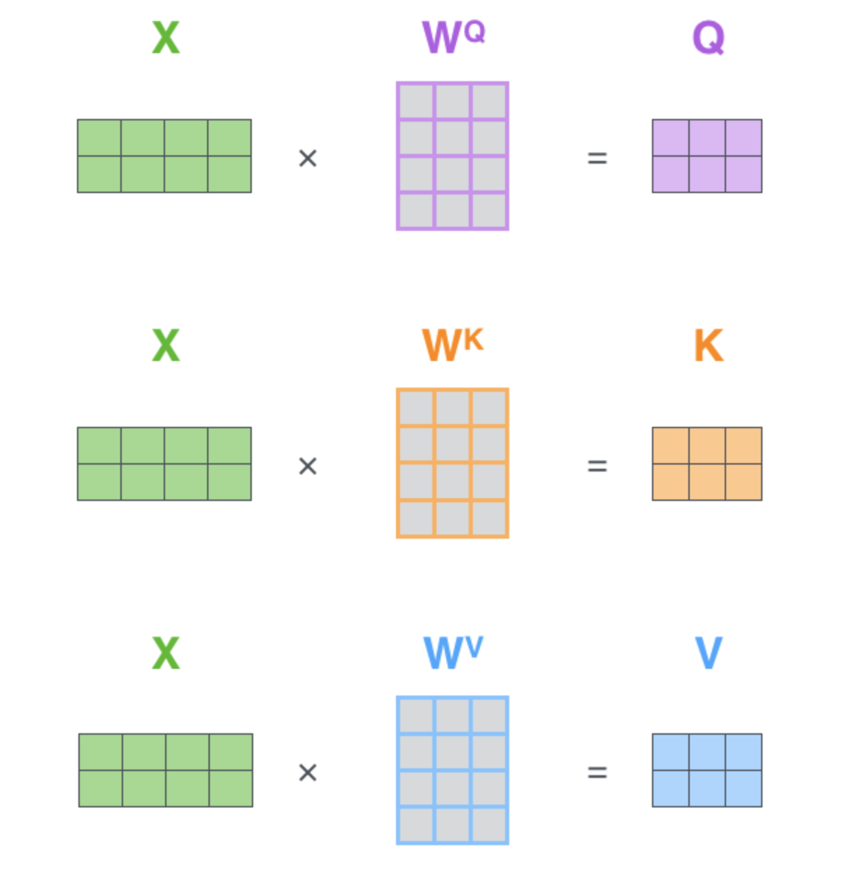
注意:这里的linear_k, linear_q, linear_v是相互独立、权重($W^Q$, $W^K$, $W^V$)是不同的,通过训练可得到。得到query(Q),key(K),value(V)之后按照下面的公式计算attention(Q, K, V):
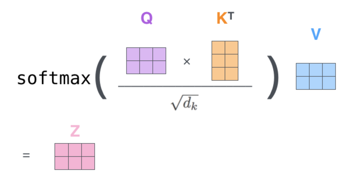
这里Z就是attention(Q, K, V)。
(1) 这里$d_k=d_{model}/h = 512/8 = 64$。
(2) 为什么要用$\sqrt{d_k}$ 对 $QK^T$进行缩放呢?
$d_k$实际上是Q/K/V的最后一个维度,当$d_k$越大,$QK^T$就越大,可能会将softmax函数推入梯度极小的区域。
(3) softmax之后值都介于0到1之间,可以理解成得到了 attention weights。然后基于这个 attention weights 对 V 求 weighted sum 值 Attention(Q, K, V)。
Multi-Head-Attention 就是将embedding之后的X按维度$d_{model}=512$ 切割成$h=8$个,分别做self-attention之后再合并在一起。
源码如下:
class MultiHeadedAttention(nn.Module):
    def __init__(self, h, d_model, dropout=0.1):
        "Take in model size and number of heads."
        super(MultiHeadedAttention, self).__init__()
        assert d_model % h == 0
        self.d_k = d_model // h
        self.h = h
        self.linears = clones(nn.Linear(d_model, d_model), 4)
        self.attn = None
        self.dropout = nn.Dropout(p=dropout)

    def forward(self, query, key, value, mask=None):
        """
        实现MultiHeadedAttention。
           输入的q,k,v是形状 [batch, L, d_model]。
           输出的x 的形状同上。
        """
        if mask is not None:
            # Same mask applied to all h heads.
            mask = mask.unsqueeze(1)
        nbatches = query.size(0)

        # 1) 这一步qkv变化:[batch, L, d_model] ->[batch, h, L, d_model/h]
        query, key, value = \
            [l(x).view(nbatches, -1, self.h, self.d_k).transpose(1, 2)
                   for l, x in zip(self.linears, (query, key, value))]

        # 2) 计算注意力attn 得到attn*v 与attn
        # qkv :[batch, h, L, d_model/h] -->x:[b, h, L, d_model/h], attn[b, h, L, L]
        x, self.attn = attention(query, key, value, mask=mask, dropout=self.dropout)
        # 3) 上一步的结果合并在一起还原成原始输入序列的形状
        x = x.transpose(1, 2).contiguous().view(nbatches, -1, self.h * self.d_k)
        # 最后再过一个线性层
        return self.linears[-1](x)
4.1.2 Add & Norm
class LayerNorm(nn.Module):
    """构造一个layernorm模块"""
    def __init__(self, features, eps=1e-6):
        super(LayerNorm, self).__init__()
        self.a_2 = nn.Parameter(torch.ones(features))
        self.b_2 = nn.Parameter(torch.zeros(features))
        self.eps = eps

    def forward(self, x):
        "Norm"
        mean = x.mean(-1, keepdim=True)
        std = x.std(-1, keepdim=True)
        return self.a_2 * (x - mean) / (std + self.eps) + self.b_2


class SublayerConnection(nn.Module):
    """Add+Norm"""
    def __init__(self, size, dropout):
        super(SublayerConnection, self).__init__()
        self.norm = LayerNorm(size)
        self.dropout = nn.Dropout(dropout)

    def forward(self, x, sublayer):
        "add norm"
        return x + self.dropout(sublayer(self.norm(x)))
注意:几乎每个sub layer之后都会经过一个归一化,然后再加在原来的输入上。这里叫残余连接。
4.2 Feed-Forward Network
# Position-wise Feed-Forward Networks
class PositionwiseFeedForward(nn.Module):
    "实现FFN函数"
    def __init__(self, d_model, d_ff, dropout=0.1):
        super(PositionwiseFeedForward, self).__init__()
        self.w_1 = nn.Linear(d_model, d_ff)
        self.w_2 = nn.Linear(d_ff, d_model)
        self.dropout = nn.Dropout(dropout)

    def forward(self, x):
        return self.w_2(self.dropout(F.relu(self.w_1(x))))
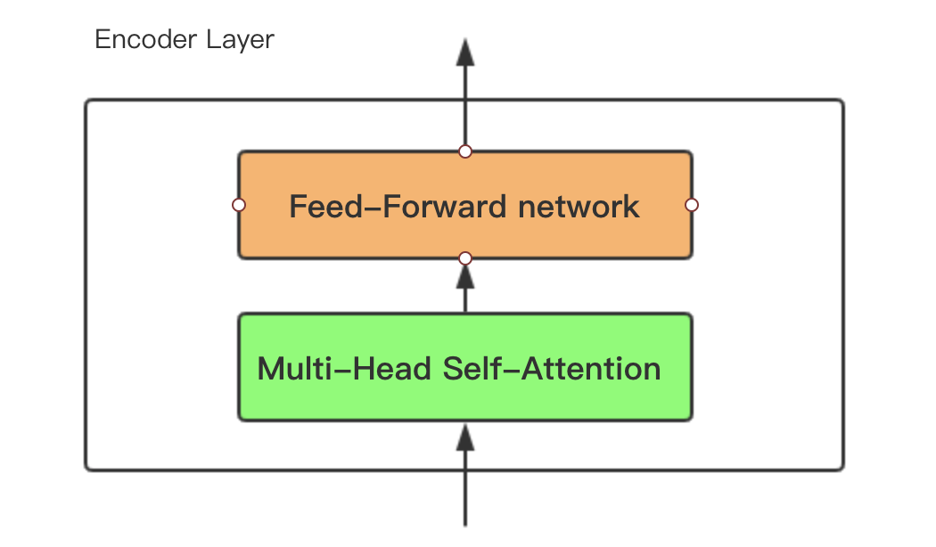
总的来说Encoder 是由上述小encoder layer 6个串行叠加组成。encoder sub layer主要包含两个部分:
- SubLayer-1 做 Multi-Headed Attention
- SubLayer-2 做 Feed Forward Neural Network
来看下Encoder主架构的代码:
def clones(module, N):
    "产生N个相同的层"
    return nn.ModuleList([copy.deepcopy(module) for _ in range(N)])

class Encoder(nn.Module):
    """N层堆叠的Encoder"""
    def __init__(self, layer, N):
        super(Encoder, self).__init__()
        self.layers = clones(layer, N)
        self.norm = LayerNorm(layer.size)

    def forward(self, x, mask):
        "每层layer依次通过输入序列与mask"
        for layer in self.layers:
            x = layer(x, mask)
        return self.norm(x)
5 Decoder
Decoder的代码主要结构:
# Decoder部分
class Decoder(nn.Module):
    """带mask功能的通用Decoder结构"""
    def __init__(self, layer, N):
        super(Decoder, self).__init__()
        self.layers = clones(layer, N)
        self.norm = LayerNorm(layer.size)

    def forward(self, x, memory, src_mask, tgt_mask):
        for layer in self.layers:
            x = layer(x, memory, src_mask, tgt_mask)
        return self.norm(x)
Decoder子结构(Sub layer):
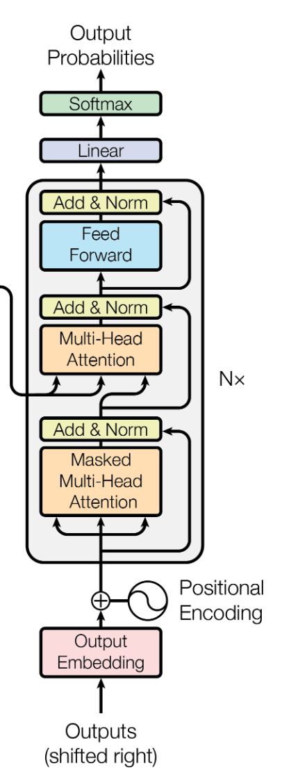
Decoder 也是N=6层堆叠的结构。被分为3个 SubLayer,Encoder与Decoder有三大主要的不同:
(1)Decoder SubLayer-1 使用的是 “Masked” Multi-Headed Attention 机制,防止为了模型看到要预测的数据,防止泄露。
(2)SubLayer-2 是一个 Encoder-Decoder Multi-head Attention。
(3) LinearLayer 和 SoftmaxLayer 作用于 SubLayer-3 的输出后面,来预测对应的 word 的 probabilities 。
5.1 Mask-Multi-Head-Attention
tensor([[[1, 0, 0, 0, 0, 0, 0, 0, 0, 0],
         [1, 1, 0, 0, 0, 0, 0, 0, 0, 0],
         [1, 1, 1, 0, 0, 0, 0, 0, 0, 0],
         [1, 1, 1, 1, 0, 0, 0, 0, 0, 0],
         [1, 1, 1, 1, 1, 0, 0, 0, 0, 0],
         [1, 1, 1, 1, 1, 1, 0, 0, 0, 0],
         [1, 1, 1, 1, 1, 1, 1, 0, 0, 0],
         [1, 1, 1, 1, 1, 1, 1, 1, 0, 0],
         [1, 1, 1, 1, 1, 1, 1, 1, 1, 0],
         [1, 1, 1, 1, 1, 1, 1, 1, 1, 1]]], dtype=torch.uint8)
def subsequent_mask(size):
    """
    mask后续的位置,返回[size, size]尺寸下三角Tensor
    对角线及其左下角全是1,右上角全是0
    """
    attn_shape = (1, size, size)
    subsequent_mask = np.triu(np.ones(attn_shape), k=1).astype('uint8')
    return torch.from_numpy(subsequent_mask) == 0
5.2 Encoder-Decoder Multi-head Attention
class DecoderLayer(nn.Module):
    "Decoder is made of self-attn, src-attn, and feed forward (defined below)"
    def __init__(self, size, self_attn, src_attn, feed_forward, dropout):
        super(DecoderLayer, self).__init__()
        self.size = size
        self.self_attn = self_attn
        self.src_attn = src_attn
        self.feed_forward = feed_forward
        self.sublayer = clones(SublayerConnection(size, dropout), 3)

    def forward(self, x, memory, src_mask, tgt_mask):
        "将decoder的三个Sublayer串联起来"
        m = memory
        x = self.sublayer[0](x, lambda x: self.self_attn(x, x, x, tgt_mask))
        x = self.sublayer[1](x, lambda x: self.src_attn(x, m, m, src_mask))
        return self.sublayer[2](x, self.feed_forward)
注意:self.sublayer[1](x, lambda x: self.src_attn(x, m, m, src_mask)) 这行就是Encoder-Decoder Multi-head Attention。
query = x,key = m, value = m, mask = src_mask,这里x来自上一个 DecoderLayer,m来自 Encoder的输出。
5.3 Linear and Softmax to Produce Output Probabilities
这部分的代码实现:
class Generator(nn.Module):
    """
    Define standard linear + softmax generation step。
    定义标准的linear + softmax 生成步骤。
    """
    def __init__(self, d_model, vocab):
        super(Generator, self).__init__()
        self.proj = nn.Linear(d_model, vocab)

    def forward(self, x):
        return F.log_softmax(self.proj(x), dim=-1)
在训练过程中,模型没有收敛得很好时,Decoder预测产生的词很可能不是我们想要的。这个时候如果再把错误的数据再输给Decoder,就会越跑越偏。这个时候怎么办?
(1)在训练过程中可以使用 “teacher forcing”。因为我们知道应该预测的word是什么,那么可以给Decoder喂一个正确的结果作为输入。
(2)除了选择最高概率的词 (greedy search),还可以选择是比如 “Beam Search”,可以保留topK个预测的word。 Beam Search 方法不再是只得到一个输出放到下一步去训练了,我们可以设定一个值,拿多个值放到下一步去训练,这条路径的概率等于每一步输出的概率的乘积。
6 Transformer的优缺点
6.1 优点
(1)每层计算复杂度比RNN要低。
(2)可以进行并行计算。
(3)从计算一个序列长度为n的信息要经过的路径长度来看, CNN需要增加卷积层数来扩大视野,RNN需要从1到n逐个进行计算,而Self-attention只需要一步矩阵计算就可以。Self-Attention可以比RNN更好地解决长时依赖问题。当然如果计算量太大,比如序列长度N大于序列维度D这种情况,也可以用窗口限制Self-Attention的计算数量。
(4)从作者在附录中给出的栗子可以看出,Self-Attention模型更可解释,Attention结果的分布表明了该模型学习到了一些语法和语义信息。
6.2 缺点
在原文中没有提到缺点,是后来在Universal Transformers中指出的,主要是两点:
(1)实践上:有些RNN轻易可以解决的问题transformer没做到,比如复制string,或者推理时碰到的sequence长度比训练时更长(因为碰到了没见过的position embedding)。
(2)理论上:transformers不是computationally universal(图灵完备),这种非RNN式的模型是非图灵完备的的,无法单独完成NLP中推理、决策等计算问题(包括使用transformer的bert模型等等)。
7 References
1 http://jalammar.github.io/illustrated-transformer/
2 https://zhuanlan.zhihu.com/p/48508221
3 https://zhuanlan.zhihu.com/p/47063917