Explanation of the structure and formula of RNN, GRU and LSTM

Based on Wu Enda's video and symbol regulations, this article introduces the structure and formula of RNN/GRU/LSTM, focusing on explaining the forward and back propagation process of RNN, especially the back propagation of RNN. I think it is relatively easy to understand . A little bit of personal experience, this part is difficult to understand in general, you can follow a teacher or a post that speaks clearly, and read it carefully.

[1] A brief introduction to RNN

First of all, why is this new structure of RNN needed?

The biggest difference between it and the previous multi-layer perceptron and convolutional neural network is that it is a sequence model, the nodes between the hidden layers are no longer connected but connected, and the input of the hidden layer includes not only the input The output of the layer also includes the output of the hidden layer at the previous moment.

For MLP or CNN, give some training data, these data are independent and unrelated to each other, but in reality some are related to time, such as the prediction of the next moment of the video, the prediction of the content of the front and back of the document, etc. These The performance of the algorithm is not satisfactory, and the serial network structure of RNN is very suitable for time series data, which can maintain the dependencies in the data.

What is the general structure of RNN?

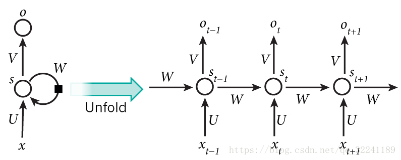
The figure below shows the general structure of RNN. The right side is expanded according to time. Through the connection on the hidden layer, the network state at the previous moment can be transmitted to the current moment, and the state at the current moment can also be passed to the next moment.

[2] Forward propagation of RNN

The network structure of RNN Here, I will use the symbol system in Wu Enda's course. I personally think that Li Hongyi can make people understand what RNN is used for from an overall perspective, and intuitively understand some of its ideas. Wu Enda The details are more detailed, and will be explained in depth from the structure and derivation. Li Mu prefers to give a brief introduction, but the advantage is that he can talk about code and answer questions.

Start with the simple case, assuming there is only one hidden layer, and the input sequence length is equal to the output sequence.

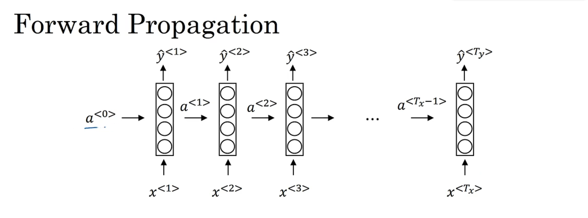
$x^{<1>},...,x^{<9>}$ is the input sequence,$x^{<i>}$ is a vector, superscript$i$ representative$i$ time steps,$a^{<t>}$ indicates the output of the hidden layer, and the circles in the box represent the hidden layer. (It can also be seen that there are connections between nodes on the same layer, which is different from ordinary fully connected networks, which only have connections between layers)

When performing forward propagation, first by $x^{<1>}$ 计算 $a^{<1>}$ ，计算式为：$$a^{<1>}=g(W_{aa}{a}^{<0>}+W_{ax}{x}^{<1>}+b_a)$$ According to this formula, it can be seen that the calculation of theiia < i > a^{<i>}$for\; i$ time steps$a^{<i>}$ used theiiInput x < i > x^{<i>}$for\; i$ time steps$x^{<i>}$ and the memory a of the previous time step$a^{<i-1>}$ , here is the first time step,$a^{<0>Wheredoes}$ it come from? Generally, a vector of all 0s is used instead. If there is no W aaa < i > W_{aa}a^{<i>}in the formula$W_{aa}{a}^{The\; <i>}$ part is the same as the structure of the multi-layer perceptron. The activation function here generally uses tanh or relu.

由 $a^{<1>}$ 计算 ${\hat{y}}^{The\; expression\; of\; <1>}$ is as follows:$${\hat{y}}^{<1>}=g(W_y{a}^{<1>}+b_y)$$ The activation function here should be determined according to the specific task. If it is a binary classification, sigmoid is generally used. If it is multi-classification, softmax is generally used.

Similarly, then start to calculate $a^{<2>}$ 和 ${\hat{y}}^{<2>}$ , for the more general case, i.e., computing$a^{<t>}$ 和 ${\hat{y}}^{<t>}$ 的表达式为：$$a^{<t>}=g(W_{aa}{a}^{<t-1>}+W_{ax}{x}^{<t>}+b_a)$$ $${\hat{y}}^{<t>}=g(W_y{a}^{<t>}+b_y)$$ For each calculation step,$W_{aa}$The city is the same, $W_y，b_a，b_y$Also, is a shared parameter for all time steps.

A simplification of the formula here is introduced in Wu Enda's video. Put $$a^{<t>}=g(W_{aa}{a}^{<t-1>}+W_{ax}{x}^{<t>}+b_a)$$ 改写为$$a^{<t>}=g(W_a[a^{<t-1>},x^{<t>}]+b_a)$$ $W_a$Commander $W_{aa}$和$W_{ax}$Glue left and right, give an example to understand:

Suppose $x^{<t>}$ is a 1000-dimensional vector,$a^{<t-1>}$ is a 100-dimensional vector, then$W_{aa}$is a 100×100 matrix, $W_{ax}$is a 100×1000 matrix.

Simplified $a^{<t-1>}$和$x^{<t>}$ put together to become a 1100-dimensional vector,$W_a$It is a matrix of 100 × 1100, which is relatively simple to write, and is exactly the same as the original operation result.

Before introducing backpropagation, first define the loss function, using the cross-entropy loss function: $$L^{<t>}({\hat{y}}^{<t>},y^{<t>})=-y^{<t>}log{\hat{y}}^{<t>}-(1-y^{<t>})log(1-{\hat{y}}^{<t>})$$This is the loss at the t-th time step, and the loss for the entire sequence is the sum of the t losses.

[3] Backpropagation BPTT of RNN

The backpropagation of RNN is called Backpropagation through time (BPTT), that is, backpropagation through time, that is, from the last time step to the previous time step one by one, and the chain rule is used repeatedly like ordinary neural networks. For convenience, the following derivations are superscripted ${}^{<t>is\; writtenas}$ subscript${}_t$

The first is the output layer parameter $W_y$,define $b_t=W_y{a}_t$, represents the state where the hidden layer multiplies the weight matrix to the output layer, but has not yet passed through the activation function (the bias item is ignored here, in fact, it is the same whether it is present or not, and the subsequent derivation will not affect it): ∂ L t ∂ W ya = $$\frac{\partial L_t}{\partial W_y}=\frac{\partial L_t}{\partial {\hat{y}}_t}\frac{\partial {\hat{y}}_t}{\partial W_y}=\frac{\partial L_t}{\partial {\hat{y}}_t}\frac{\partial {\hat{y}}_t}{\partial {\beta }_t}\frac{\partial {\beta }_t}{\partial W_y}$$
After that $W_{aa}$和$W_{ax}$, these two need to consider the gradient at the current moment (the gradient passed down from the loss function at the current moment t) and the gradient at the next moment (the gradient passed down from the time t+1) when updating the gradient. For convenience, then Define two variables: $z_t=W_{ax}{x}_t+W_{aa}{a}_{t-1}$, is the hidden layer node of the tth time step (accepting the input $x_t$and at − 1 a_{t-1} at time t-1$a_{t-1}$) but has not yet passed through the activation function. Let $d_t$Indicates the moment $z_t$ 接受到的梯度。$$d_t=\frac{\partial L_t}{\partial \widehat{y_t}}\frac{\partial \widehat{y_t}}{\partial a_t}\frac{\partial a_t}{\partial z_t}+d_{t+1}\frac{\partial z_{t+1}}{\partial a_t}\frac{\partial a_t}{\partial z_t}$$Find $d_t$After that, it is easy to find $L_t$VS $W_{aa}$和$W_{ax}$ 的导数：$d_t{a}_{t-1}^T,d_t{x}_t^T$

---

Give a specific small example to see how to calculate it. Assuming that there are only three time steps in total, the forward propagation process of the data is as follows (here $z,\beta$ has a bias term, but it does not affect):

$W_y$The gradient of is not counted because it is relatively simple. First look at the third time step, look at $L_3$VS $W_{aa}$ 的影响：$$\frac{\partial L_3}{\partial W_{aa}}=\frac{\partial L_3}{\partial \widehat{y_3}}\frac{\partial \widehat{y_3}}{\partial {\beta }_3}\frac{\partial {\beta }_3}{\partial a_3}\frac{\partial a_3}{\partial z_3}\frac{\partial z_3}{\partial W_{aa}}$$Remove the last item on the right side of the equal sign $\frac{\partial z_3}{\partial W_{aa}}$It is the δ 3 \delta_3 we stipulated above$d_3$, the reason why this is specified is for the convenience of calculation and description, because the missing item will be expanded later.

The gradient is passed back to the second time step, not only must be considered by $L_2$The calculated gradient and the gradient from time t=3. First consider $L_2$ 的：$$\frac{\partial L_2}{\partial W_{aa}}=\frac{\partial L_2}{\partial \widehat{y_2}}\frac{\partial \widehat{y_2}}{\partial {\beta }_2}\frac{\partial {\beta }_2}{\partial a_2}\frac{\partial a_2}{\partial z_2}\frac{\partial z_2}{\partial W_{aa}}$$Then $L_3$经$a_3$pass to $a_2$Here, it is actually the above $\frac{\partial L_3}{\partial W_{aa}}$ 继续往下链式求导：$$\frac{\partial L_3}{\partial \widehat{y_3}}\frac{\partial \widehat{y_3}}{\partial {\beta }_3}\frac{\partial {\beta }_3}{\partial a_3}\frac{\partial a_3}{\partial z_3}\frac{\partial z_3}{\partial a_2}\frac{\partial a_2}{\partial z_2}\frac{\partial z_2}{W_{aa}}=d_3\frac{\partial z_3}{\partial a_2}\frac{\partial a_2}{\partial z_2}\frac{\partial z_2}{W_{aa}}$$So the total gradient accepted at the second time step is the sum of the two.

Come to the first time step, although it is not drawn on the picture, there is actually $a_0$. Last $W_{aa}$The update is $L_3$Incoming gradient + $L_2$Incoming gradient + $L_1$incoming gradient.

vsW $W_{ax}$The same is true for the calculation of , so I won't say more about it. In essence, it is still a chain derivation that has been passed down. Or to put it this way, take $L_t$As a parameter to be updated such as $W_{aa}$The multi-layer nested composite function, using the chain rule to derive to the innermost layer of our parameters to be updated, the feeling of peeling off layer by layer.

[4] Gradient disappearance and gradient explosion of RNN

Gradient disappearance means that the result of many derivative multiplications will be very close to 0. The gradient disappearance makes RNN not good at capturing long-distance dependencies. For example, for a very deep network, forward propagation of the network from left to right and then backpropagation, from the output $\hat{y}$The obtained gradient is difficult to propagate back, it is difficult to affect the weight of the previous layer, and it is difficult to affect the calculation of the previous layer. An output is mainly related to the nearby input, and it is basically difficult to be affected by the input at the front of the sequence. This is because no matter what the output is, whether it is right or wrong, it is difficult for this area to backpropagate to the sequence. In the front part, it is also difficult for the network to adjust the calculations in front of the sequence. This is a shortcoming of the basic RNN algorithm.

Gradient disappearance is the primary problem when training RNN. Although gradient explosion will also occur, gradient explosion is obvious, because exponentially large gradients will make your parameters extremely large, so that your network parameters collapse. So the gradient explosion is easy to spot, because the parameters will be so large that they will collapse, and you will see a lot of NaN, or not a number, which means that your network calculations have numerical overflow. If you find problems with exploding gradients, one solution is to use gradient pruning. Gradient pruning means to observe your gradient vector, if it is larger than a certain threshold, scale the gradient vector to ensure that it is not too large, this is the method of pruning by some maximum value (that is, when the gradient you calculate exceeds the threshold c Or when it is less than the threshold -c, the gradient at this time is set to c or -c).

[5] Gated recurrent unit GRU

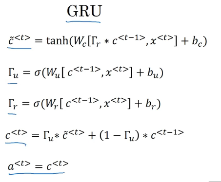
GRU changes the hidden layer of RNN so that it can better capture deep connections and improve the problem of gradient disappearance. This is the GRU formula given in the video, and then I will explain it in detail:

(1) First, the original $a^{<t>}$ use c here$c^{<t>}$ to indicate, refers to the$The\; output\; value\; of\; the\; hidden\; layer\; at\; t$ time steps, naturally,$W_a$Also changed to $W_c$ . $c$ means cell, which is understood as "memory cell", that is, it has memory ability and can maintain the value of the previous cell, thereby alleviating the problem of gradient disappearance/long-distance dependence.

(2) except $c^{<t>}$ , also added${\tilde{c}}^{<t>asa}$ candidate value. As you can see later, the original calculation$a^{The\; formula\; of\; <t>}$ gets the candidate value${\tilde{c}}^{<t>}$ , after some processing will finally get$c^{<t>}$ 。

(3) There are two "gates", and the "gate" uses $\Gamma$ means,$\Gamma$ is covered with sigmoid, its value is between 0 and 1, and the probability is relatively close to 0 or 1, so as to achieve control. The two doors are:

• $C_r$: correlation gate, controlling ${\tilde{c}}^{<t>}$ 和 $c^{}$The magnitude of the correlation between${}^{<}$${}^t$${}^{-}$${}^1$${}^{>\; ,\; r\; means\; relevant}$
• $C_u$: Update gate, which controls whether the value of the memory cell is updated, that is, whether to use ${\tilde{c}}^{<t>}$ 更新 $c^{<t>}$ ，u 表示 update

---

Now, to think through the whole process, $c^{<t-1>}$ is the hidden layer output of the last time step, first by$c^{<t-1>}$ 和 $x^{<t>}$ Calculate the candidate value${\tilde{c}}^{<t>}$：$${\tilde{c}}^{<t>}=tanh\left(W_c\right[C_r\ast c^{<t-1>}，x^{<t>}]+b_c)$$ This calculated value should have been$a^{<t>}$ (or$c^{<t>}$ ), but now it is just a candidate value, and some operations are required to determine the final$c^{<t>.\_}$ _ Note that here$c^{<t-1>}$ is also multiplied by a$C_r$, if $C_r$Close to 0, it means that the correlation with the hidden layer output of the previous time step is very small, otherwise it is very large. $C_r$The value of is equivalent to "the degree of door opening", controlling $c^{<t-1>}$ Influence on the next time step.

Then calculate $c^{<t>}$：$$c^{<t>}=C_u\ast {\tilde{c}}^{<t>}+(1-C_u)\ast c^{<t-1>}$$如果$C_u$Close to 1, then $c^{<t>}$ is approximately equal to the candidate value, if$C_u$Close to 0, then $c^{<t>}$ is equal to the output of the previous time step, which is equivalent to no update, and the previous value is maintained, which is similar to "memory".

---

It is not difficult to see that RNN is $C_r=1,C_u=1$ when the special case of the GRU. But I also think, only$C_u$Ok? It is updated when it is equal to 1, and it is not updated when it is equal to 0. Why there is $C_r$? This is because over the years researchers have tried many, many different possible ways to design these units, to try to make the neural network have deeper connections, to try to produce a wider range of influence, and to solve the problem of gradient disappearance, GRU It is one of the most commonly used versions by researchers, and it has also been found to be very robust and practical on many different problems. (Probably because, doing so is good in the experiment?

[6] Long short-term memory neural network LSTM

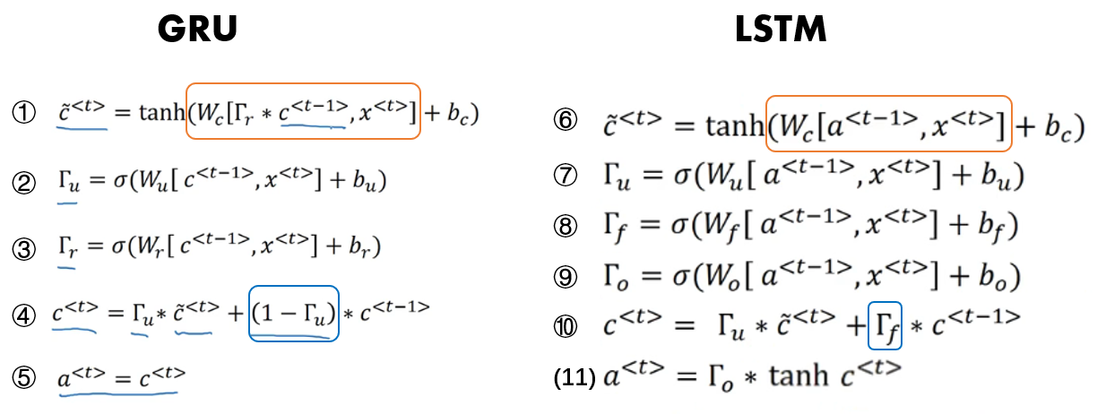
LSTM is a more general and powerful form of GRU. Now let's talk about the structure of LSTM. First is the memory cell c, use ${\tilde{c}}^{<t>}=tanh(W_c[a^{<t-1>}，x^{<t>}]+b_c)$ to update its candidate value. Note that in LSTM we no longer have$a^{<t>}=c^{<t>}$ case, now we specifically use$a^{<t>}$ 或者$a^{<t-1>}$ , and do not use$C_r$, that is, the relevant gate.

Like GRU there is an update gate $C_u$and the parameter W u W_u representing the update$W_u$, but not only one update gate controls, Γ u \Gamma_u in ④$C_u$和$1-C_u$Represented by different terms to allow for a more flexible structure. Therefore, let $C_f$Determine1 $1-C_u$ ，$C_f$Represents the forget gate, controlling how much to forget $c^{<t-1>}$ . So this gives the memory cell the option to maintain the old value$c^{<t-1>}$ or just add a new value${\tilde{c}}^{<t>}$ , so a separate update gate$C_u$and forget gate $C_f$ .

Then there is a new output gate $C_o$ ，将 $a^{<t>}=c^{<t>}$ 变成 $a^{<t>}=C_o\ast c^{<t>}$

We use graphs for a more intuitive understanding:

由 $a^{<t-1>}$ 和 $x^{<t>}$ DefinitionsΓ$C_f,C_u,C_o$The value at time t, and ${\tilde{c}}^{<t>}$，然后 $c^{<t-1>}\ast C_f$，${\tilde{c}}^{<t>}\ast C_u$, the two are added to get $c^{<t>}$， $c^{<t>}$ multiplied by Γ o \Gamma_o​​after tanh$C_o$Get hidden layer output $a^{<t>}$.

[7] Comparing GRU and LSTM

When should we use GRU? When to use LSTM? There is no uniform guideline here. In fact, in the history of deep learning, LSTM appeared earlier, and GRU was invented only recently. It may have originated from the simplification made by Pavia in the more complex LSTM model.

The advantage of GRU is that this is a simpler model , so it is easier to create a larger network, and it only has two gates, and it runs faster computationally, and then it can expand the size of the model, and the effect is also good.

But LSTM is more powerful and flexible because it has three gates instead of two. If you want to pick one to use, I think LSTM has historically been a more preferred choice, so if you have to pick one, I feel that most people today will still try LSTM as the default choice.

[8] Summary

RNN is a sequence model that is often used for tasks such as named entity recognition, machine translation, and text generation. Its typical feature is that the output of the hidden layer at a certain moment is not only related to the input data at that moment , but also related to the output of the hidden layer at the previous moment , but RNN has the problems of gradient disappearance and long-term dependence . GRU adds two gates on the basis of RNN: correlation gate and update gate. GRU can form memory and decide whether to update at each moment. RNN can be regarded as a special case of GRU. And LSTM is a more powerful and general version.