Neural Network and Deep Learning Lab Report
1. Experiment name
Numpy implements fully connected neural network
2. Experimental requirements
Implementing fully connected neural networks with python's numpy module. The network structure is an input layer, a hidden layer, and an output layer. The activation function of the hidden layer is the Relu function, the activation function of the output layer is the softmax function, and the loss function is the cross entropy.
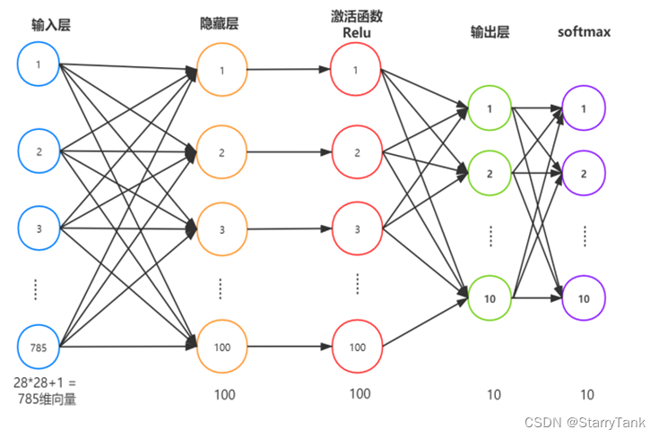
Figure 1 - Schematic diagram of network structure
3. The purpose of the experiment
Through learning the basic principles of feedforward neural network (network structure, loss function, parameter learning), use numpy to realize neural network, and further deepen the understanding of neural network. Master the principles and methods of neural networks.
4. Experimental process
4.1 Feedforward neural network
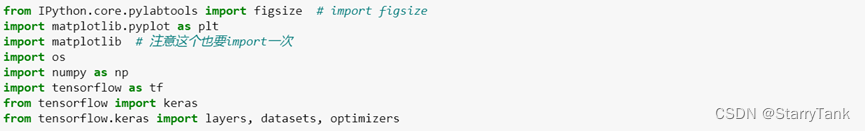
4.1.1 Environment configuration
Required packages are: numpy, tensorflow, keras
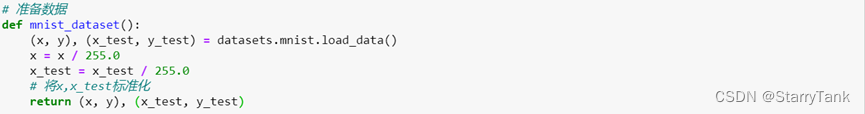
4.1.2 Prepare data
Using the handwritten font data set mnist, the training data set contains 60,000 samples, and the test data set contains 10,000 samples. Each picture is composed of 28x28 pixels, and each pixel is represented by a gray value. Here, the 28x28 Pixels are unwrapped into a 1D vector and each pixel value is normalized, labeled 0-9.
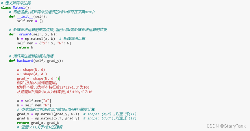
4.1.3 Defining the matrix multiplication class
The matrix multiplication class includes forward propagation to calculate the input matrix X of the hidden layer and backpropagation to calculate the gradient of the weight matrix W and the input matrix X, which is calculated from the gradient grad_y of the output matrix Y to obtain the gradient of the loss about the X matrix and the W matrix , grad_x and grad_w
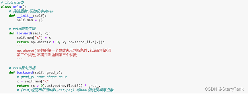
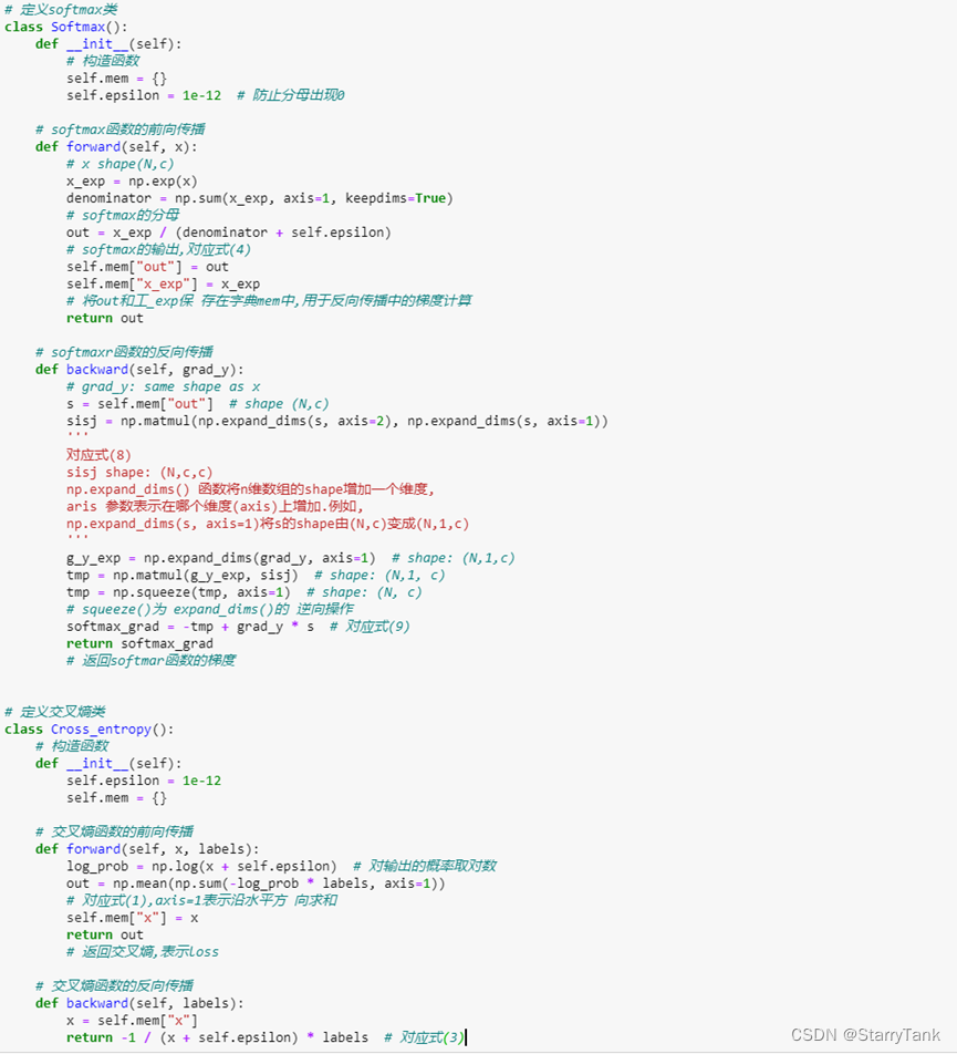
4.1.3 Define Relu class, Softmax class, cross entropy class
The Relu class includes forward propagation to calculate the activation value as the input matrix X of the next layer, and back propagation to calculate the loss function gradient according to the gradient grad_y of the output value Y. The Softmax class is used as the activation function of the output layer, and the cross-entropy class is used as the calculation of the loss function.
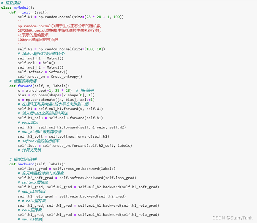
4.1.4 Define the model
Including the initialization of the network weight matrix, the forward propagation and back propagation of the model to calculate the gradient of the loss on the weight matrix W
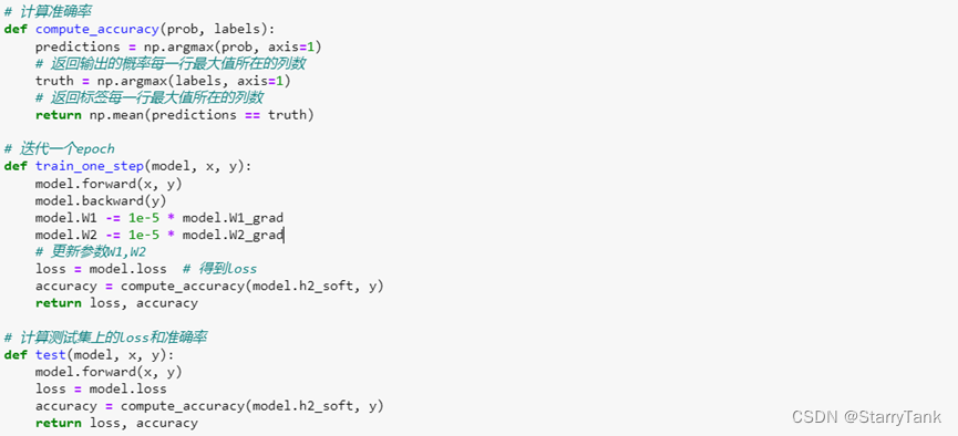
4.1.5 Calculation of training set accuracy, iteration, calculation of test set loss and accuracy function
The accuracy is calculated according to the Softmax value, the loss is calculated according to the cross-entropy loss function, and the weight matrix is updated according to the gradient value.
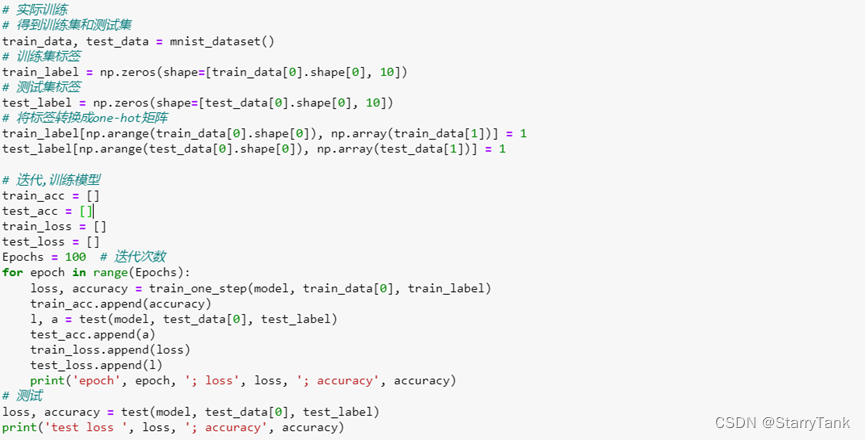
4.1.5 Model training and evaluation
Divide the training set and test set, label processing, set the number of iterations, record the accuracy and loss value.
4.2 Change neural network topology, activation rules and learning algorithms
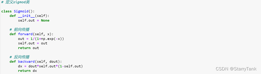
4.2.1 Change the activation function (sigmoid activation function)
The original code uses the Relu function, the advantages of Relu: The gradient of the relu function is constant in the part greater than 0, so there will be no gradient disappearance. For the sigmod function, the gradient in the positive and negative saturation regions is close to 0, which may cause the gradient to disappear. The derivative calculation of the Relu function is faster, so it is much faster to converge than Sigmod when using gradient descent. Relu Cons: Relu death problem. Advantages of Sigmod: It has good explanatory properties, and outputs the combination of linear functions as a probability between 0 and 1. Disadvantages of Sigmodu: The activation function has a large amount of calculation. When backpropagating to find the gradient, the derivation involves division. During backpropagation, the derivatives on both sides of the saturation region are likely to be 0, that is, the gradient is prone to disappear, so that the training of the deep network cannot be completed. Customize the Sigmoid function class to change the activation function, the code is as follows:
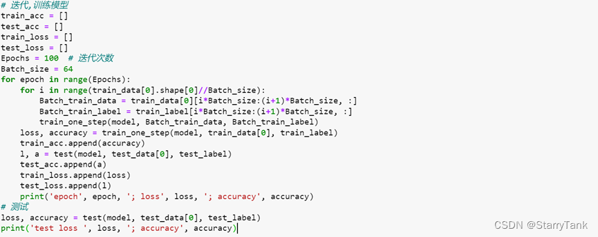
4.2.2 Changing the learning algorithm (mini-batch gradient descent)
The batch gradient descent algorithm is used in the original code, and the cross-entropy loss function of all samples needs to be calculated each time. When the number of samples is too large, the calculation amount is large. The disadvantage of the stochastic gradient descent method is that it cannot use the parallel computing power of the computer. The mini-batch gradient descent algorithm (Mini-Batch Gradient Descent) is a compromise between batch gradient descent and stochastic gradient descent. At each iteration, a small number of samples are selected to compute gradients and update parameters. This can not only take into account the advantages of the stochastic gradient descent method, but also improve the training efficiency. In practical applications, the mini-batch gradient descent algorithm has the advantages of fast convergence and low computational overhead. The specific code is as follows:
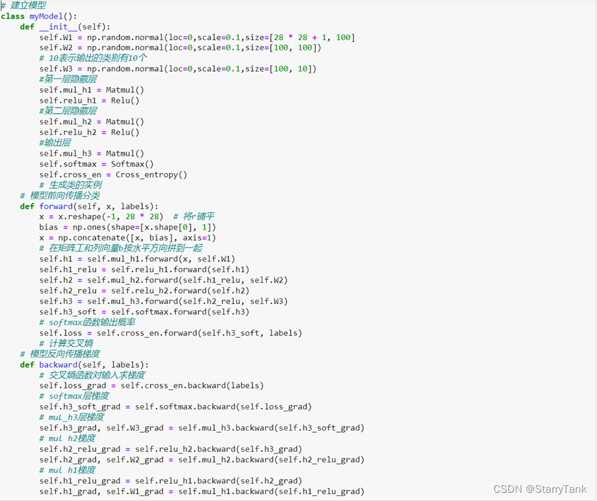
4.2.3 Change the network structure (increase the number of layers and neurons)
In order to make the model more accurate, the number of network layers is increased, from one hidden layer to two hidden layers, and the number of neurons is 100. The specific code is as follows:
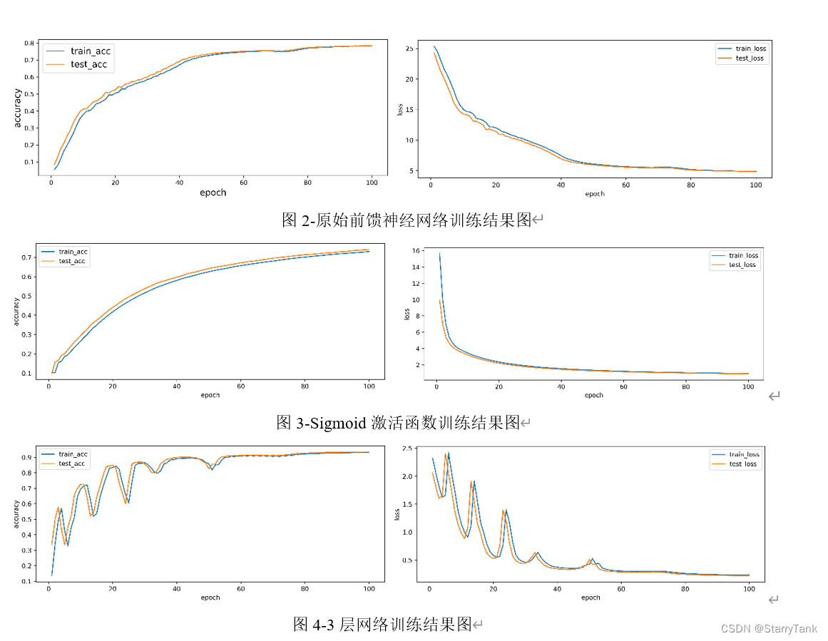
5. Experimental results
6. Experimental summary
In this experiment, the construction and training process of the feedforward neural network was realized through numpy, and the derivation of mathematical theory was realized through code, which deepened the understanding of the neural network. The ability to learn models before and after, combined with theoretical knowledge, has a lot to gain. According to the comparative analysis of the experimental results, the following experiences are obtained:
(1) As the number of network layers deepens and the number of neurons increases, the fitting ability of the model will become stronger.
(2) The convergence speed of the Sigmoid activation function is not as good as that of the Relu function. The reason should be that the two ends of the Sigmoid function are saturated, and the problem of gradient disappearance is prone to occur. The effect in this experiment is average.
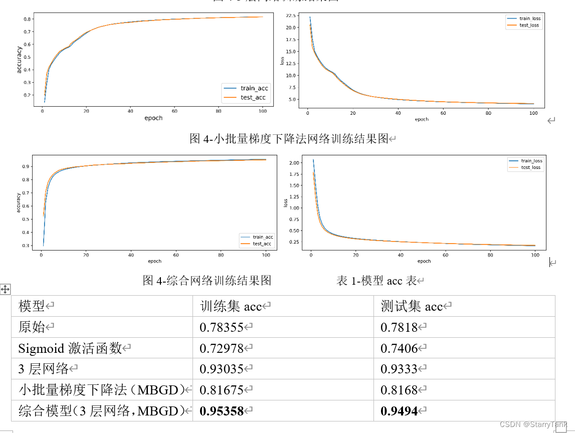
(3) The mini-batch gradient descent algorithm converges much faster than the batch gradient descent algorithm, and the accuracy of the model is higher.
(4) The comprehensive model adopts activation function, 3-layer neural network (2 hidden layers), and small batch gradient descent algorithm. The convergence speed of the model is fast, and it has basically converged when eopch is 20, and the accuracy rate is the highest. In the training set and 0.95358 and 0.9494 on the test set, respectively.
In the course of the experiment, we also encountered problems. When the neural network is deepened or the number of neurons is increased, the Softmax function of the output layer will overflow during calculation, but when inputting, the pixel value has been standardized. By consulting the data and and After discussion, the students found that it may be because the value of the weight initialization is large. With the increase of the number of neural network layers, the forward propagation continues to accumulate, resulting in a large final output value. After the exponential operation, the value is too large to cause overflow. The solution There are: reduce the initialization weight value and increase the learning rate appropriately, and make changes from the Softmax function calculation.