It is said that dimensionality reduction is a data processing method often used in the field of machine learning, so before this column officially starts the topic of deep learning, we will first introduce several commonly used dimensionality reduction methods (PCA, KPCA, t-SNE, MDS, etc.) and MATLAB accomplish.
There are already good articles about the principle of PCA on Zhihu, so I will not explain it in detail here. Students who want to know more can read here:
How to explain what is PCA (Principal Component Analysis) in an easy-to-understand manner?
What I want to do here is mainly from the perspective of practical application that many people have not mentioned too much. I will give you two vivid cases to introduce when PCA dimensionality reduction is used, whether it is easy to use, and how to use.
1. The basic concept of PCA
Principal Component Analysis (PCA) is widely used in data dimensionality reduction [1] .
Through a series of variance-maximizing projections, PCA can obtain the eigenvectors whose eigenvalues are arranged from large to small, and then select the dimension to intercept the corresponding matrix according to the needs.
Let me give two examples below to illustrate the common applications and usage methods of PCA.
2. Case 1: Dimensionality reduction, clustering and classification
Here is an introduction to the iris data set, which is one of the frequent visitors in machine learning. The data set consists of 150 instances, and its feature data includes four: sepal length, sepal width, petal length, and petal width. There are three kinds of irises in the data set, called Setosa, Versicolor, and Virginica, as shown in the figure below:

That is to say, the dimension of this set of data is 150*4, and the data is labeled . ( Having a label means that each instance we know its corresponding category)
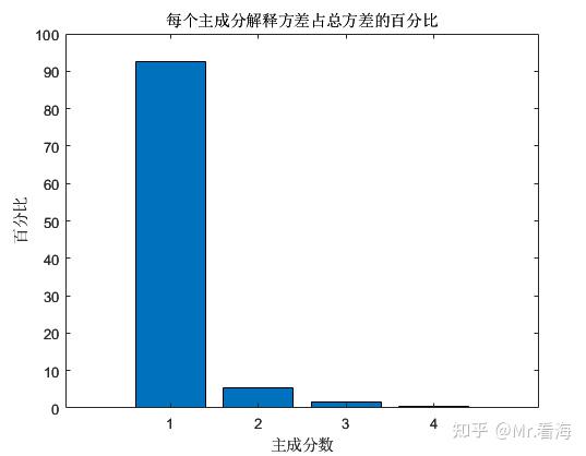
At this time, we perform PCA dimensionality reduction, and we can get the percentage of variance explained by each principal component in the total variance. This value can be used to represent the amount of information contained in each principal component. From the calculation results, the first principal component and The sum of the percentages of the second principal component has exceeded 97%, and the sum of the percentages of the first three principal components has exceeded 99%.
We can plot the distribution of dimensionality reduction data when the data is reduced to two-dimensional and three-dimensional:
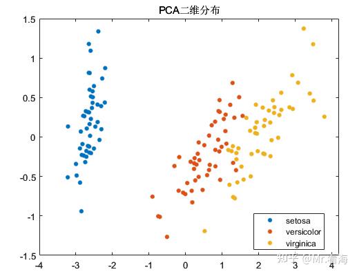
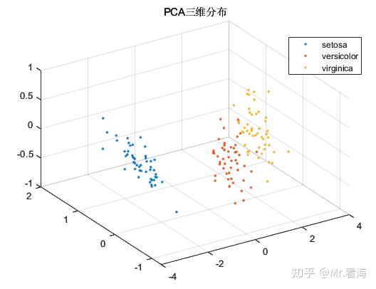
Although the original intention of the PCA algorithm is dimensionality reduction rather than clustering, the data after PCA dimensionality reduction is often used as input data for machine learning, and the distribution of the data after dimensionality reduction is checked while the data is reduced. For pattern recognition/ It is still very beneficial to determine the intermediate state of the classification task. To put it bluntly, it is also excellent to put these pictures in the paper to enrich the content.
In this application scenario, the main purpose of data dimensionality reduction is actually to solve the problem that the data features are too large. In this example, there are only 4 features, so it is not very obvious. Many times we are faced with tens, hundreds or even more feature dimensions. These features contain a lot of redundant information, making the calculation task very heavy, and the difficulty of parameter adjustment will be greatly increased. At this time, it is very necessary to add a step of data dimensionality reduction.
3. Case 2: Health indicators in life expectancy prediction
In the previous article, PCA was used to characterize life expectancy health indicators:
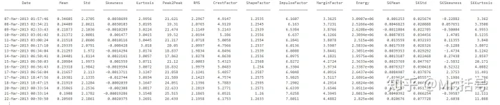
In this case, the features used include those of the original signal: "Mean"; "Std"; "Skewness"; "Kurtosis"; "Peak2Peak","RMS"; "CrestFactor"; "ShapeFactor"; "ImpulseFactor"; "MarginFactor"; "Energy".
And for spectral kurtosis: "Mean"; "Std"; "Skewness"; "Kurtosis".
There are 15 feature values in total, and a feature table with a size of 50*15 can be obtained within 50 days. Part of the data in the table is as follows:
但是做寿命预测与做分类不同,在寿命预测任务中,需要将上述特征融合成单一指标,作为表征当前设备健康状态的量化数值,也就是所谓的健康指标。此时就需要将15维特征降为1维,并用这1维数据代表退化特征。此时画出来的退化过程如下:
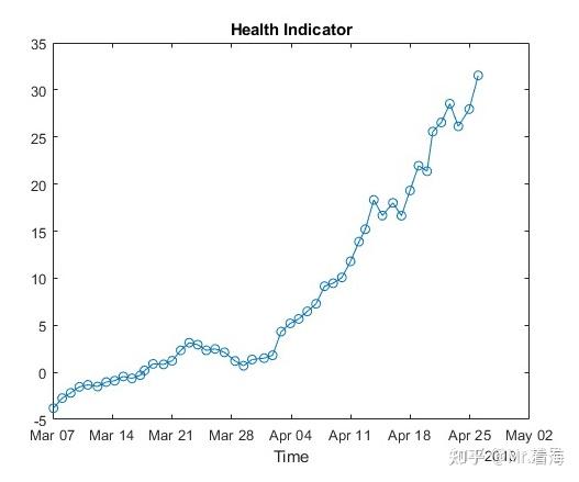
有了这张图,后续的寿命预测就可以以此为基准,将复杂的问题转换为时间序列预测了。
四、MATLAB的PCA降维快速实现
PCA算法在MATLAB中有官方函数,名字就叫做pca,熟悉编程的同学可以直接调用。
对于不熟悉MATLAB编程,或者希望更简洁的方法实现PCA降维,并同时绘制出相关图片的同学,则可以考虑使用本专栏封装的函数,它可以实现:
1.输入数据的行列方向纠正。是的,MATLAB的pca函数对特征矩阵的输入方向是有要求的,如果搞不清,程序可以帮你自动纠正。
options.autoDir='on';%是否进行自动纠错,'on'为是,否则为否。开启自动纠错后会智能调整数据的行列方向。2.指定输出的维度。也就是降维之后的维度,当然这个数不能大于输入数据的特征维度。
options.NumDimensions=3;%降维后的数据维度3.数据归一化。你可以选择在PCA之前,对特征数据进行归一化,这也只需要设置一个参数。
options.Standardize=false;%输入数据是否进行标准化,false (默认) | true 4.绘制特征分布图和成分百分比图。在降维维度为2或者3时,可以绘制特征分布图,当然你也可以选择设置不画图,图个清静。
figflag='on';%是否画图,'on'为画图,'off'为不画,只有NumDimensions为2或者3时起作用,3以上无法画图设置好这些配置参数后,只需要调用下边这行代码:
[pcaVal,explained,coeff]=khPCA(data,options,species,figflag);%pcaVal为降维后的数据矩阵就可以绘制出这样两张图:

如果要绘制二维图,把options.NumDimensions设置成2就好了。
不过上述是知道标签值species的情况,如果不知道标签值,设置species=[]就行了,此时画出来的分布图是单一颜色的。
上述代码秉承了本专栏一向的易用属性,功能全部集中在khPCA函数里了,这个函数更详细的介绍如下:
function [pcaVal,explained,coeff,PS] = khPCA(data,options,species,figflag)
% 对数据进行PCA降维并且画图
% 输入:
% data:拟进行降维的数据,data维度为m*n,其中m为特征值种类数,n为每个特征值数据长度
% options:一些与pca降维有关的设置,使用结构体方式赋值,比如 options.autoDir = 'on',具体包括:
%              -autoDir:是否进行自动纠错,'on'为是,否则为否。开启自动纠错后会智能调整数据的行列方向。
%              -NumDimensions:降维后的数据维度,默认为2,注意NumDimensions不能大于data原本维度
%              -Standardize:输入数据是否进行标准化,false (默认) | true
%
% species:分组变量,可以是数组、数值向量、字符数组、字符串数组等,但是需要注意此变量维度需要与Fea的组数一致。该变量可以不赋值,调用时对应位置写为[]即可
%          例如species可以是[1,1,1,2,2,2,3,3,3]这样的数组,代表了Fea前3行数据为第1组,4-6行数据为第2组,7-9行数据为第三组。
%          关于此species变量更多信息,可以查看下述链接中的"Grouping variable":
%          https://ww2.mathworks.cn/help/stats/gscatter.html?s_tid=doc_ta#d124e492252
%
% figflag:是否画图,'on'为画图,'off'为不画,只有NumDimensions为2或者3时起作用,3以上无法画图
% 输出:
% pcaVal:主成分分数,即经过pca分析计算得到的主元,每一列是一个主元
% explained:每个主成分解释方差占总方差的百分比,以列向量形式返回。
% coeff:主成分系数,由于data*coeff=score,所以当有一组新的数据data2想要以同样的主元坐标系进行降维时,可以使用data2*coeff得到,然后截取相应的列
% 但如果options.Standardize设置为true,则需要采用下述指令实施同步归一化及降维: mapminmax('apply',data2,PS)*coeff
% PS:数据归一化的相关参数,只有在options.Standardize设置为true时会返回该参数
需要上边这个函数文件以及测试代码的同学,可以在下边链接获取:
参考
^跟着迪哥学 Python数据分析与机器学习实战