One article introduces the quick understanding and application of the PCA algorithm, and this chapter talks about KPCA.
The KPCA method, like the PCA method, has a solid theoretical foundation. A lot of materials can be found in papers and on the Internet for related theories. Therefore, this article focuses on the quick understanding and application of the method. The parameter setting methods that may be more concerned are explained, so as to achieve the purpose of getting started quickly.
1. The basic concept of KPCA
The Kernel Principal Component Analysis (KPCA) method is an improvement of the PCA method. It can be easily seen from the name that the difference lies in the "kernel". The purpose of using the kernel function: to construct a complex nonlinear classifier.
Kernel Methods (Kernel Methods) is a non-parametric statistical learning method widely used in the field of machine learning. It can be used for classification, regression, clustering and other tasks, and is widely used in computer vision, natural language processing, bioinformatics and other fields. For example, "core" is also one of the core concepts in the SVM method.
The core idea of the kernel method is to transform the data points in the input space into a feature space through mapping, so that the data points in the feature space can be processed and analyzed more easily. And this kind of mapping is usually realized by kernel function (Kernel Function).
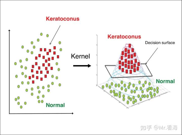
Schematic diagram of conversion from low latitude to high latitude, source: https://entokey.com/artificial-intelligence-in-keratoconus/
It should be noted that the kernel function itself does not explicitly define the high-dimensional feature space, but uses kernel techniques to realize the mapping of data from low-dimensional space to high-dimensional feature space. This method can greatly reduce the computational complexity, and at the same time can deal with nonlinear problems, because it can map the original data into a nonlinear feature space, so that the data points in the feature space can be more easily detected by linear classifiers or regressors. deal with.
Let me give two examples (consistent with the previous PCA article) to illustrate the common applications and usage methods of KPCA, as well as some differences from the KPCA method.
2. Why data dimensionality reduction
Data dimensionality reduction refers to mapping high-dimensional data into a low-dimensional space while retaining important information in the data. This dimensionality reduction operation can help us better understand and process data, reduce computational complexity, and improve the efficiency and accuracy of machine learning algorithms.
As an example, suppose we have a demographics dataset that contains various information about 10,000 individuals, such as age, gender, occupation, income, etc. These information can be expressed as a matrix of 10,000 rows x 10 columns, that is, each person's information is represented by a 10-dimensional vector. However, these dimensions can be redundant and incur high computational cost when performing machine learning analysis. Therefore, we can consider performing dimension reduction operations on these data and map them to a lower-dimensional space, such as 3-dimensional or 2-dimensional. In this new low-dimensional space, we can still retain important information in the data, such as the difference between different occupations, the correlation between age and income, etc., but the computational complexity will be greatly reduced, which is more suitable for machine learning Algorithmic processing.
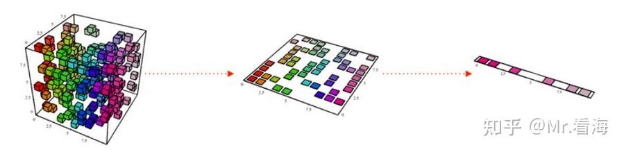
Source: https://blog.csdn.net/danwenxuan/article/details/76647940 , the demonstration is the reduction from 3 dimensions to 1 dimension, and the above population example is descending from 10 dimensions
Data dimensionality reduction has many uses, here are some of the common ones:
1. Data visualization: In high-dimensional data, it is difficult for the human visual system to intuitively understand the characteristics and relationships of the data. By reducing the data to a two-dimensional or three-dimensional space, we can more easily visualize and explore the data.
2. Remove redundant features: In some applications, there may be a large number of redundant features in the data set, which are not helpful for modeling and may even affect model performance. Through data dimensionality reduction, we can remove redundant features and improve modeling efficiency and performance.
3. Accelerated algorithms: In some algorithms, such as clustering and classification, high-dimensional data will lead to a sharp increase in computational complexity. Through data dimensionality reduction, we can reduce high-dimensional data to low-dimensional, thereby speeding up the operation of the algorithm.
4. Reduce storage and computing costs: As the data set continues to grow, storage and computing costs will increase dramatically. Through data dimensionality reduction, we can reduce the dimensionality of data to a lower level, thereby reducing storage and computing costs.
三、为什么用KPCA
KPCA是PCA的一种扩展形式,它可以有效地应对非线性数据,并且具有以下几个优点:
1.更好的数据可分性
KPCA在将数据映射到高维空间后,能够更好地区分不同类别的数据,提高了数据的可分性。举例来说,如果数据集是一个螺旋形状,那么使用 PCA 很难将这个数据集分离成两个类别,因为 PCA 只能处理线性数据结构。但是,如果使用 KPCA,可以将数据映射到高维空间中,使得数据在新的空间中变得线性可分,从而更容易进行分类。
2.善于处理非线性数据
与PCA只能处理线性数据不同,KPCA可以处理非线性数据。KPCA使用核函数,将原始数据映射到一个高维的特征空间上,该空间具有更强的表达能力,能够处理非线性关系。在这个高维特征空间中,我们可以使用PCA来提取主成分,再将它们映射回原始空间。这样就可以在原始空间中实现非线性变换,从而更好地处理非线性数据。对于许多实际问题有很好的应用前景,例如图像处理和模式识别。
3.更加灵活的使用方式
KPCA的核函数还可以通过调整参数来进一步调整模型的复杂度和鲁棒性。因此,相对于PCA,KPCA具有更多的灵活性和可调性,可以更好地适应不同的数据场景和需求。
四、KPCA中的几个重要参数
1.核函数(Kernel Function)
核函数用于将原始数据映射到一个高维空间中,从而能够更好地区分数据。常见的核函数包括线性核(linear)、多项式核(poly)、高斯核(gaussian)等,径向基核(RBF)是高斯核的另一种表达形式,本质上是相同的。不同的核函数可以对数据进行不同类型的变换,从而影响降维效果。
2.核函数参数(Kernel Function Parameter)
核函数通常包含一个或多个参数,例如高斯核就有一个标准差参数。这些参数影响了核函数变换的程度,可以通过交叉验证等方法来确定最佳参数值。
2.1 高斯核函数中的gamma(γ)参数:高斯核函数定义为  ,其中,γ是高斯核函数的一个超参数。它控制了数据点在高维空间中的分布情况。当γ越大时,高斯核函数会使得数据点在高维空间中的分布更加集中,因此,降维后的数据将更容易区分。常见的取值范围为
  到
到  。
。
2.2 多项式核函数中的r和d参数:多项式核函数定义为  ,其中,r是常数项,d是多项式的阶数,这两个参数控制了多项式核函数的形状。
r是平移参数,它的作用是将多项式核函数平移一定的距离,使得更多的数据被映射到高维空间。
d的取值范围为1到10之间的整数。如果d取值过大,会导致过拟合的问题,如果取值过小,则可能会欠拟合数据。
3.降维后的维度(Number of Components)
该参数是需要同学们自己指定的,在实际使用中通常需要结合实际应用场景进行设置。如果不知道该怎样设置,可以结合各个成分的贡献度进行筛选。贡献度越高,表示该主成分对数据的解释能力越强,因此在选择主成分时可以根据其贡献度进行排序,选择贡献度较高的主成分作为保留的特征。
比如上边人口统计的例子中,经kpca融合后得到的特征就会按照贡献度从大到小排序,我们可以取总贡献度之和达到85%或者90%(自定)的前几个特征作为降维后的特征数据,而这个特征数量就是降维后的维度。
下边我们举例说明一下。
五、案例:降维、聚类与分类
举一个PCA中介绍过的例子。
这里介绍一下鸢尾花数据集,鸢尾花在机器学习里是常客之一。数据集由具有150个实例组成,其特征数据包括四个:萼片长、萼片宽、花瓣长、花瓣宽。数据集中一共包括三种鸢尾花,分别叫做Setosa、Versicolor、Virginica,就像下图:

也就是说这组数据的维度是150*4,数据是有标签的。(有标签是指每个实例我们都知道它对应的类别)
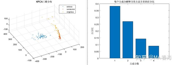
此时我们进行KPCA降维,可以得到每个主成分解释方差占总方差的百分比,这个数值可以用以表示每个主成分中包含的信息量,从计算结果上来看,第1个主成分和第2个主成分的百分比之和已经超过95%,前三个主成分百分比之和更是超过了99%。此时我们就可以按照贡献率来筛选降维后的维度了,比如设置总贡献度能达到99%以上,那么就把降维维度设置为2即可。

我们可以绘制一下数据降到二维和三维时,降维数据的分布情况:
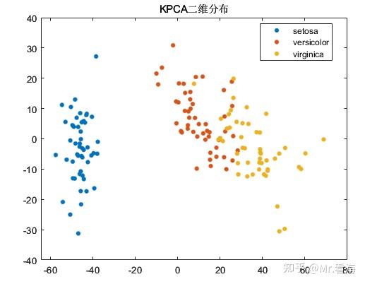

尽管PCA算法的初衷是降维而非聚类,不过由于KPCA降维后的数据常常会用做机器学习的输入数据,在数据降维的同时查看降维后数据的分布情况,对于模式识别/分类任务的中间状态确定还是十分有益的,再直白些说,这些图片放在论文里丰富一下内容也是极好的。
在这种应用场景下,数据降维的最主要目的其实还是解决数据特征过于庞大的问题,这个例子中特征只有4个,所以还不太明显。很多时候我们面对的是几十上百乃至更多的特征维度,这些特征中包含着大量冗余信息,使得计算任务变得非常繁重,调参的难度和会大大增加。此时加入一步数据降维就是十分有必要的了。
六、MATLAB的KPCA降维快速实现
KPCA算法在MATLAB中还没有官方函数,不过已经有前辈造出了轮子。大家可以在下边链接下载和使用:
对于不熟悉MATLAB编程,或者希望更简洁的方法实现KPCA降维,并同时绘制出相关图片的同学,则可以考虑使用本专栏封装的函数,它可以实现:
1.输入数据的行列方向纠正。是的,MATLAB的pca函数对特征矩阵的输入方向是有要求的,如果搞不清,程序可以帮你自动纠正。
options.autoDir='on';%是否进行自动纠错,'on'为是,否则为否。开启自动纠错后会智能调整数据的行列方向。2.指定输出的维度。也就是降维之后的维度,当然这个数不能大于输入数据的特征维度。
options.NumDimensions=3;%降维后的数据维度3.数据归一化。你可以选择在PCA之前,对特征数据进行归一化,这也只需要设置一个参数。
options.AutoScale=false;%输入数据是否进行标准化,false (默认) | true 4.绘制特征分布图和成分百分比图。在降维维度为2或者3时,可以绘制特征分布图,当然你也可以选择设置不画图,图个清静。
figflag='on';%是否画图,'on'为画图,'off'为不画,只有NumDimensions为2或者3时起作用,3以上无法画图5.相关超参数设置。
options.gamma=2;%超参数gamma的数值,默认为2,只对gaussian核有效options.r=1;%超参数r的数值,默认为1,只对polynomial核有效options.d=2;%超参数d的数值,默认为2,只对polynomial核有效设置好这些配置参数后,只需要调用下边这行代码:
[kpcaVal,explained]=khKPCA(data,options,species,figflag);%kpcaVal为降维后的数据矩阵,explained为各成分贡献度就可以绘制出这样两张图:
绘制三维分布图
如果要绘制二维图,把options.NumDimensions设置成2就好了。绘制出来是这样:

绘制二维分布图
不过上述是知道标签值species的情况,如果不知道标签值,设置species=[]就行了,此时画出来的分布图是单一颜色的。
上述代码秉承了本专栏一向的易用属性,功能全部集中在khPCA函数里了,这个函数更详细的介绍如下:
[kpcaVal,explained] = khKPCA(data,options,species,figflag);
% 执行KPCA操作,并实现画图
% 依赖函数:KernelPca.m,原始代码见:https://github.com/kitayama1234/MATLAB-Kernel-PCA
% 输入:
% data:拟进行降维的数据,data维度为m*n,其中m为特征值种类数,n为每个特征值数据长度
% options:一些与kpca降维有关的设置,使用结构体方式赋值,比如 options.autoDir = 'on',具体包括:
%              -autoDir:是否进行自动纠错,'on'为是,否则为否。开启自动纠错后会智能调整数据的行列方向。
%              -NumDimensions:降维后的数据维度,默认为2,注意NumDimensions不能大于data原本维度
%              -kernel: kernel类型选择('linear', 'gaussian', or 'polynomial'),默认为linear
%              -gamma:超参数gamma的数值,默认为2
%              -r:超参数r的数值,默认为1
%              -d:超参数d的数值,默认为2
%              -AutoScale:是否进行标准化,True或False,默认为False
%
% species:分组变量,可以是数组、数值向量、字符数组、字符串数组等,但是需要注意此变量维度需要与Fea的组数一致。该变量可以不赋值,调用时对应位置写为[]即可
%          例如species可以是[1,1,1,2,2,2,3,3,3]这样的数组,代表了Fea前3行数据为第1组,4-6行数据为第2组,7-9行数据为第三组。
%          关于此species变量更多信息,可以查看下述链接中的"Grouping variable":
%          https://ww2.mathworks.cn/help/stats/gscatter.html?s_tid=doc_ta#d124e492252
%
% figflag:是否画图,'on'为画图,'off'为不画,只有NumDimensions为2或者3时起作用,3以上无法画图
% 输出:
% pcaVal:主成分分数,即经过pca分析计算得到的主元,每一列是一个主元
% explained:每个主成分解释方差占总方差的百分比,以列向量形式返回。
需要上边这个函数文件以及测试代码的同学,可以在下边链接获取:
附录
linear核函数 :

gaussian核函数 :

polynomial核函数 :