Locally weighted linear regression for prediction (code included)

The purpose of regression is to predict a numerical target value. The simplest method is linear regression. Linear regression means that you can multiply the input items by some constants and add the results to get the output. However, a problem with linear regression is the potential for underfitting because it seeks an unbiased estimate with the smallest mean squared error. If the model is underfitting, the best prediction effect will not be obtained. So some methods allow to introduce some bias in the estimation, thereby reducing the mean square error of the forecast.

One of these methods is Locally Weighted Linear Regression (LWLR). In this algorithm, we assign a certain weight to each point near the point to be predicted, and then perform ordinary regression based on the minimum mean square error on this subset. Like kNN, this algorithm needs to select the corresponding data subset in advance for each prediction. The algorithm solves the regression coefficient w in the following form:

$\hat{w}=(X^{T}WX)^{-1}X^{T}Wy$

where w is a matrix used to assign weights to each data point.

LWLR uses "kernels" (similar to those in support vector machines) to give higher weights to nearby points. The type of kernel can be freely selected. The most commonly used kernel is the Gaussian kernel. The weights corresponding to the Gaussian kernel are as follows:

$w(i,i)=exp(\frac{|x^{(i)}-x|}{-2k^{2}})$

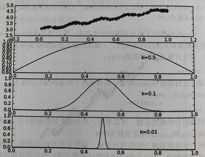
This constructs a weight matrix w with only diagonal elements, and the closer the point x is to x(i), the larger w(i,i) will be. The above formula contains a parameter k that needs to be specified by the user, which determines how much weight is given to nearby points. This is also the only parameter that needs to be considered when using LWLR. The relationship between parameter k and weight is shown in the following figure:

Use locally weighted linear regression for data fitting, and the MATLAB code is as follows:

clear ;  
close all;  
% x = [1:50].';  
% y = [4554 3014 2171 1891 1593 1532 1416 1326 1297 1266 ...  
%     1248 1052 951 936 918 797 743 665 662 652 ...  
%     629 609 596 590 582 547 486 471 462 435 ...  
%     424 403 400 386 386 384 384 383 370 365 ...  
%     360 358 354 347 320 319 318 311 307 290 ].';  
load('data');
len = 90;
y=data(:,8);
y=y(1:len,1);
x=1:len;
x=x.';

m = length(y); % store the number of training examples  
x = [ ones(m,1) x]; % Add a column of ones to x  
n = size(x,2); % number of features  
theta_vec = inv(x'*x)*x'*y;  
tau = [1 10 25];  
y_est = zeros(length(tau),length(x));  
for kk = 1:length(tau)  
    for ii = 1:length(x);  
        w_ii = exp (- (x (ii, 2) - x (:, 2)). ^ 2./(2*tau(kk)^2));  
        W = diag (w_ii);  
        theta_vec = inv(x'*W*x)*x'*W*y;  
        y_est(kk, ii) = x(ii,:)*theta_vec;  
    end
end  
  
figure;  
plot(x(:,2),y,'ks-'); hold on  
plot(x(:,2),y_est(1,:),'bp-');  
% plot(x(:,2),y_est(2,:),'rx-');  
% plot(x(:,2),y_est(3,:),'go-');  
legend('measured', 'predicted, tau=1', 'predicted, tau=10','predicted, tau=25');  
grid on;  
xlabel('Page index, x');  
ylabel('Page views, y');  
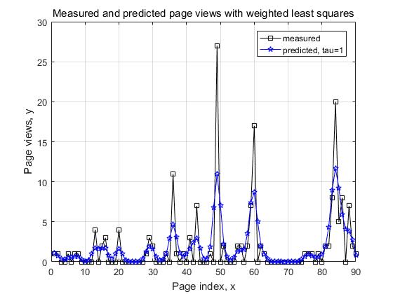
title('Measured and predicted page views with weighted least squares');

The effect is as shown in the figure:

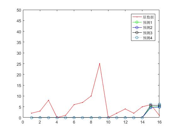
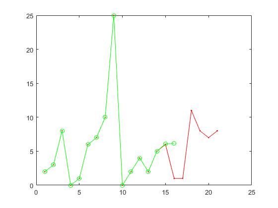
Using locally weighted linear regression for data prediction, the results are shown in the figure:

Locally weighted linear regression for prediction (code included)

Guess you like