目录
一、深层神经网络

二、深层神经网络的前向传播和反向传播


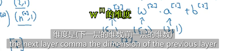
三、核对矩阵维数
拿出一张纸,计算各个矩阵的维度


四、参数和超参数


作业:


#! /usr/bin/env python
# -*- coding: utf-8 -*-

"""
============================================
时间:2021.8.19
作者:手可摘星辰不去高声语
文件名:搭建多层神经网络.py
功能:【吴恩达课后编程作业】01 - 神经网络和深度学习 - 第四周编程作业
1、Ctrl + Enter      在下方新建行但不移动光标;
2、Shift + Enter     在下方新建行并移到新行行首;
3、Shift + Enter     任意位置换行
4、Ctrl + D          向下复制当前行
5、Ctrl + Y         删除当前行
6、Ctrl + Shift + V  打开剪切板
7、Ctrl + /          注释(取消注释)选择的行;
8、Ctrl + E       可打开最近访问过的文件
9、Double Shift + /  万能搜索
============================================
"""

import numpy as np
import h5py
import matplotlib.pyplot as plt
import 第4周.编程题.testCases
from 第4周.编程题 import lr_utils
from 第4周.编程题.dnn_utils import sigmoid, sigmoid_backward, relu, relu_backward

# 指定随机种子
np.random.seed(1)


# 1. 初始化网络参数  layers_dims代表各个层的节点数
def initialize_parameters_deep(layers_dims):
    """
    此函数是为了初始化多层网络参数而使用的函数。
    参数:
        layers_dims - 包含我们网络中每个图层的节点数量的列表

    返回:
        parameters - 包含参数“W1”,“b1”,...,“WL”,“bL”的字典:
                     W1 - 权重矩阵,维度为(layers_dims [1],layers_dims [1-1])
                     bl - 偏向量,维度为(layers_dims [1],1)
    """
    np.random.seed(3)
    parameters = {}
    L = len(layers_dims)

    for l in range(1, L):
        parameters["W" + str(l)] = np.random.randn(layers_dims[l], layers_dims[l - 1]) / np.sqrt(layers_dims[l - 1])
        parameters["b" + str(l)] = np.zeros((layers_dims[l], 1))

    # 确保我要的数据的格式是正确的
    assert (parameters["W" + str(l)].shape == (layers_dims[l], layers_dims[l - 1]))
    assert (parameters["b" + str(l)].shape == (layers_dims[l], 1))

    return parameters


# 2.前向传播
# 2.1 线性部分
def linear_forward(A, W, b):
    """
    实现前向传播的线性部分

    参数:
        A - 来自上一层(或输入数据)的激活,维度为(上一层的节点数量,示例的数量)
        W - 权重矩阵,numpy数组,维度为(当前图层的节点数量,前一图层的节点数量)
        b - 偏向量,numpy向量,维度为(当前图层节点数量,1)

    返回:
         Z - 激活功能的输入,也称为预激活参数
         cache - 一个包含“A”,“W”和“b”的字典,存储这些变量以有效地计算后向传递
    """
    Z = np.dot(W, A) + b
    assert (Z.shape == (W.shape[0], A.shape[1]))
    cache = (A, W, b)

    return Z, cache


# 2.2 线性激活部分
def linear_activation_forward(A_prev, W, b, activation):
    """
    实现LINEAR-> ACTIVATION 这一层的前向传播

    参数:
        A_prev - 来自上一层(或输入层)的激活,维度为(上一层的节点数量,示例数)
        W - 权重矩阵,numpy数组,维度为(当前层的节点数量,前一层的大小)
        b - 偏向量,numpy阵列,维度为(当前层的节点数量,1)
        activation - 选择在此层中使用的激活函数名,字符串类型,【"sigmoid" | "relu"】

    返回:
        A - 激活函数的输出,也称为激活后的值
        cache - 一个包含“linear_cache”和“activation_cache”的字典,我们需要存储它以有效地计算后向传递
    """

    Z, linear_cache = linear_forward(A_prev, W, b)

    if activation == "sigmoid":
        A, activation_cache = sigmoid(Z)
    elif activation == "relu":
        A, activation_cache = relu(Z)

    assert (A.shape == (W.shape[0], A_prev.shape[1]))
    cache = (linear_cache, activation_cache)

    return A, cache


# 2.3 多层模型:结合线性求和与激活函数
def L_model_forward(X, parameters):
    """
    实现[LINEAR-> RELU] *(L-1) - > LINEAR-> SIGMOID计算前向传播,也就是多层网络的前向传播,为后面每一层都执行LINEAR和ACTIVATION

    参数:
        X - 数据,numpy数组,维度为(输入节点数量,示例数)
        parameters - initialize_parameters_deep()的输出

    返回:
        AL - 最后的激活值
        caches - 包含以下内容的缓存列表:
                 linear_relu_forward()的每个cache(有L-1个,索引为从0到L-2)
                 linear_sigmoid_forward()的cache(只有一个,索引为L-1)
    """

    caches = []
    A = X
    L = len(parameters) // 2
    for l in range(1, L):
        A_prev = A
        A, cache = linear_activation_forward(A_prev, parameters['W' + str(l)], parameters['b' + str(l)], "relu")
        caches.append(cache)

    AL, cache = linear_activation_forward(A, parameters['W' + str(L)], parameters['b' + str(L)], "sigmoid")
    caches.append(cache)

    assert (AL.shape == (1, X.shape[1]))

    return AL, caches


# 3.计算成本
def compute_cost(AL, Y):
    """
    实施等式(4)定义的成本函数。

    参数:
        AL - 与标签预测相对应的概率向量,维度为(1,示例数量)
        Y - 标签向量(例如:如果不是猫,则为0,如果是猫则为1),维度为(1,数量)

    返回:
        cost - 交叉熵成本
    """
    m = Y.shape[1]
    cost = -np.sum(np.multiply(np.log(AL), Y) + np.multiply(np.log(1 - AL), 1 - Y)) / m

    cost = np.squeeze(cost)
    assert (cost.shape == ())

    return cost


# 4. 反向传播
# 4.1 线性部分
def linear_backward(dZ, cache):
    """
    为单层实现反向传播的线性部分(第L层)

    参数:
         dZ - 相对于(当前第l层的)线性输出的成本梯度
         cache - 来自当前层前向传播的值的元组(A_prev,W,b)

    返回:
         dA_prev - 相对于激活(前一层l-1)的成本梯度,与A_prev维度相同
         dW - 相对于W(当前层l)的成本梯度,与W的维度相同
         db - 相对于b(当前层l)的成本梯度,与b维度相同
    """
    A_prev, W, b = cache
    m = A_prev.shape[1]
    dW = np.dot(dZ, A_prev.T) / m
    db = np.sum(dZ, axis=1, keepdims=True) / m
    dA_prev = np.dot(W.T, dZ)

    assert (dA_prev.shape == A_prev.shape)
    assert (dW.shape == W.shape)
    assert (db.shape == b.shape)

    return dA_prev, dW, db


# 4.2 线性激活部分
def linear_activation_backward(dA, cache, activation="relu"):
    """
    实现LINEAR-> ACTIVATION层的后向传播。

    参数:
         dA - 当前层l的激活后的梯度值
         cache - 我们存储的用于有效计算反向传播的值的元组(值为linear_cache,activation_cache)
         activation - 要在此层中使用的激活函数名,字符串类型,【"sigmoid" | "relu"】
    返回:
         dA_prev - 相对于激活(前一层l-1)的成本梯度值,与A_prev维度相同
         dW - 相对于W(当前层l)的成本梯度值,与W的维度相同
         db - 相对于b(当前层l)的成本梯度值,与b的维度相同
    """
    linear_cache, activation_cache = cache
    if activation == "relu":
        dZ = relu_backward(dA, activation_cache)
        dA_prev, dW, db = linear_backward(dZ, linear_cache)
        return dA_prev, dW, db
    elif activation == "sigmoid":
        dZ = sigmoid_backward(dA, activation_cache)
        dA_prev, dW, db = linear_backward(dZ, linear_cache)
        return dA_prev, dW, db


# 4.3 多层网络反向传播
def L_model_backward(AL, Y, caches):
    """
    对[LINEAR-> RELU] *(L-1) - > LINEAR - > SIGMOID组执行反向传播,就是多层网络的向后传播

    参数:
     AL - 概率向量,正向传播的输出(L_model_forward())
     Y - 标签向量(例如:如果不是猫,则为0,如果是猫则为1),维度为(1,数量)
     caches - 包含以下内容的cache列表:
                 linear_activation_forward("relu")的cache,不包含输出层
                 linear_activation_forward("sigmoid")的cache

    返回:
     grads - 具有梯度值的字典
              grads [“dA”+ str(l)] = ...
              grads [“dW”+ str(l)] = ...
              grads [“db”+ str(l)] = ...
    """
    grads = {}
    L = len(caches)
    m = AL.shape[1]
    Y = Y.reshape(AL.shape)
    dAL = - (np.divide(Y, AL) - np.divide(1 - Y, 1 - AL))

    current_cache = caches[L - 1]
    grads["dA" + str(L - 1)], grads["dW" + str(L)], grads["db" + str(L)] = linear_activation_backward(dAL,
                                                                                                      current_cache,
                                                                                                      "sigmoid")

    for l in reversed(range(L - 1)):
        current_cache = caches[l]
        dA_prev_temp, dW_temp, db_temp = linear_activation_backward(grads["dA" + str(l + 1)], current_cache, "relu")
        grads["dA" + str(l)] = dA_prev_temp
        grads["dW" + str(l + 1)] = dW_temp
        grads["db" + str(l + 1)] = db_temp

    return grads


# 5.更新参数
def update_parameters(parameters, grads, learning_rate):
    """
    使用梯度下降更新参数

    参数:
     parameters - 包含你的参数的字典
     grads - 包含梯度值的字典,是L_model_backward的输出

    返回:
     parameters - 包含更新参数的字典
                   参数[“W”+ str(l)] = ...
                   参数[“b”+ str(l)] = ...
    """
    L = len(parameters) // 2  # 整除
    for l in range(L):
        parameters["W" + str(l + 1)] = parameters["W" + str(l + 1)] - learning_rate * grads["dW" + str(l + 1)]
        parameters["b" + str(l + 1)] = parameters["b" + str(l + 1)] - learning_rate * grads["db" + str(l + 1)]

    return parameters


# 搭建多层神经网络
def L_layer_model(X, Y, layers_dims, learning_rate=0.0075, num_iterations=3000, num_iter_avg=100, print_cost=False, isPlot=True):
    """
    实现一个L层神经网络:[LINEAR-> RELU] *(L-1) - > LINEAR-> SIGMOID。

    参数:
	    X - 输入的数据,维度为(n_x,例子数)
        Y - 标签,向量,0为非猫,1为猫,维度为(1,数量)
        layers_dims - 层数的向量,维度为(n_y,n_h,···,n_h,n_y)
        learning_rate - 学习率
        num_iterations - 迭代的次数
        print_cost - 是否打印成本值,每100次打印一次
        isPlot - 是否绘制出误差值的图谱

    返回:
     parameters - 模型学习的参数。 然后他们可以用来预测。
    """
    np.random.seed(1)
    costs = []
    running_cost = 0
    parameters = initialize_parameters_deep(layers_dims)

    for i in range(0, num_iterations):
        AL, caches = L_model_forward(X, parameters)
        cost = compute_cost(AL, Y)
        grads = L_model_backward(AL, Y, caches)
        parameters = update_parameters(parameters, grads, learning_rate)

        running_cost = running_cost + cost
        # 打印成本值,如果print_cost=False则忽略

        if print_cost:
            if i % num_iter_avg == num_iter_avg - 1:
                costs.append(running_cost / num_iter_avg)
                print("第", i+1, "次迭代,成本值为:", running_cost / num_iter_avg)
                running_cost = 0

    # 迭代完成,根据条件绘制图
    if isPlot:
        plt.plot(np.squeeze(costs))
        plt.ylabel('cost')
        plt.xlabel('iterations (per tens)')
        plt.title("Learning rate =" + str(learning_rate))
        plt.show()
    return parameters


# 加载数据集
train_set_x_orig, train_set_y, test_set_x_orig, test_set_y, classes = lr_utils.load_dataset()

train_x_flatten = train_set_x_orig.reshape(train_set_x_orig.shape[0], -1).T
test_x_flatten = test_set_x_orig.reshape(test_set_x_orig.shape[0], -1).T

train_x = train_x_flatten / 255
train_y = train_set_y
test_x = test_x_flatten / 255
test_y = test_set_y

layers_dims = [12288, 20, 7, 5, 1]  # 5-layer model
parameters = L_layer_model(train_x, train_y, layers_dims, num_iterations=2500, print_cost=True, isPlot=True)
#! /usr/bin/env python
# -*- coding: utf-8 -*-

"""
============================================
时间:2021.8.19
作者:
文件名:dnn_utils.py
功能:【吴恩达课后编程作业】01 - 神经网络和深度学习 - 第四周编程作业
1、Ctrl + Enter      在下方新建行但不移动光标;
2、Shift + Enter     在下方新建行并移到新行行首;
3、Shift + Enter     任意位置换行
4、Ctrl + D          向下复制当前行
5、Ctrl + Y         删除当前行
6、Ctrl + Shift + V  打开剪切板
7、Ctrl + /          注释(取消注释)选择的行;
8、Ctrl + E       可打开最近访问过的文件
9、Double Shift + /  万能搜索
============================================
"""


import numpy as np

def sigmoid(Z):
    """
    Implements the sigmoid activation in numpy

    Arguments:
    Z -- numpy array of any shape

    Returns:
    A -- output of sigmoid(z), same shape as Z
    cache -- returns Z as well, useful during backpropagation
    """

    A = 1/(1+np.exp(-Z))
    cache = Z

    return A, cache

def sigmoid_backward(dA, cache):
    """
    Implement the backward propagation for a single SIGMOID unit.

    Arguments:
    dA -- post-activation gradient, of any shape
    cache -- 'Z' where we store for computing backward propagation efficiently

    Returns:
    dZ -- Gradient of the cost with respect to Z
    """

    Z = cache

    s = 1/(1+np.exp(-Z))
    dZ = dA * s * (1-s)

    assert (dZ.shape == Z.shape)

    return dZ

def relu(Z):
    """
    Implement the RELU function.

    Arguments:
    Z -- Output of the linear layer, of any shape

    Returns:
    A -- Post-activation parameter, of the same shape as Z
    cache -- a python dictionary containing "A" ; stored for computing the backward pass efficiently
    """

    A = np.maximum(0,Z)

    assert(A.shape == Z.shape)

    cache = Z
    return A, cache

def relu_backward(dA, cache):
    """
    Implement the backward propagation for a single RELU unit.

    Arguments:
    dA -- post-activation gradient, of any shape
    cache -- 'Z' where we store for computing backward propagation efficiently

    Returns:
    dZ -- Gradient of the cost with respect to Z
    """

    Z = cache
    dZ = np.array(dA, copy=True) # just converting dz to a correct object.

    # When z <= 0, you should set dz to 0 as well.
    dZ[Z <= 0] = 0

    assert (dZ.shape == Z.shape)

    return dZ
#! /usr/bin/env python
# -*- coding: utf-8 -*-

"""
============================================
时间:2021.8.19
作者:
文件名:lr_utils.py
功能:【吴恩达课后编程作业】01 - 神经网络和深度学习 - 第四周编程作业
1、Ctrl + Enter      在下方新建行但不移动光标;
2、Shift + Enter     在下方新建行并移到新行行首;
3、Shift + Enter     任意位置换行
4、Ctrl + D          向下复制当前行
5、Ctrl + Y         删除当前行
6、Ctrl + Shift + V  打开剪切板
7、Ctrl + /          注释(取消注释)选择的行;
8、Ctrl + E       可打开最近访问过的文件
9、Double Shift + /  万能搜索
============================================
"""


import numpy as np

def sigmoid(Z):
    """
    Implements the sigmoid activation in numpy

    Arguments:
    Z -- numpy array of any shape

    Returns:
    A -- output of sigmoid(z), same shape as Z
    cache -- returns Z as well, useful during backpropagation
    """

    A = 1/(1+np.exp(-Z))
    cache = Z

    return A, cache

def sigmoid_backward(dA, cache):
    """
    Implement the backward propagation for a single SIGMOID unit.

    Arguments:
    dA -- post-activation gradient, of any shape
    cache -- 'Z' where we store for computing backward propagation efficiently

    Returns:
    dZ -- Gradient of the cost with respect to Z
    """

    Z = cache

    s = 1/(1+np.exp(-Z))
    dZ = dA * s * (1-s)

    assert (dZ.shape == Z.shape)

    return dZ

def relu(Z):
    """
    Implement the RELU function.

    Arguments:
    Z -- Output of the linear layer, of any shape

    Returns:
    A -- Post-activation parameter, of the same shape as Z
    cache -- a python dictionary containing "A" ; stored for computing the backward pass efficiently
    """

    A = np.maximum(0,Z)

    assert(A.shape == Z.shape)

    cache = Z
    return A, cache

def relu_backward(dA, cache):
    """
    Implement the backward propagation for a single RELU unit.

    Arguments:
    dA -- post-activation gradient, of any shape
    cache -- 'Z' where we store for computing backward propagation efficiently

    Returns:
    dZ -- Gradient of the cost with respect to Z
    """

    Z = cache
    dZ = np.array(dA, copy=True) # just converting dz to a correct object.

    # When z <= 0, you should set dz to 0 as well.
    dZ[Z <= 0] = 0

    assert (dZ.shape == Z.shape)

    return dZ


import numpy as np
import h5py


def load_dataset():
    train_dataset = h5py.File('datasets/train_catvnoncat.h5', "r")
    train_set_x_orig = np.array(train_dataset["train_set_x"][:]) # your train set features
    train_set_y_orig = np.array(train_dataset["train_set_y"][:]) # your train set labels

    test_dataset = h5py.File('datasets/test_catvnoncat.h5', "r")
    test_set_x_orig = np.array(test_dataset["test_set_x"][:]) # your test set features
    test_set_y_orig = np.array(test_dataset["test_set_y"][:]) # your test set labels

    classes = np.array(test_dataset["list_classes"][:]) # the list of classes

    train_set_y_orig = train_set_y_orig.reshape((1, train_set_y_orig.shape[0]))
    test_set_y_orig = test_set_y_orig.reshape((1, test_set_y_orig.shape[0]))

    return train_set_x_orig, train_set_y_orig, test_set_x_orig, test_set_y_orig, classes