A time series is a set of real numbers in chronological order, such as stock trading data. By analyzing the time series, it is possible to dig out the laws behind this set of series, so as to effectively predict the future data. In this part, common statistical methods based on time series will be described.
1 Use the rolling method to calculate the moving average
When the number of samples in the time series fluctuates greatly and it is not easy to analyze the future development trend, the moving average method can be used to eliminate the influence of random fluctuations. It can be said that the moving average method is a commonly used analysis method for time series. The basic idea is to calculate the average value of the specified window sequence in turn according to the time series sample data, gradually moving backward.
The moving average of stocks is a relatively common example, through which we can analyze the trend of future stock prices. Technically speaking, you can use the rolling method of pandas to calculate the moving average with a specified time window. In the following CalMA.py example, it will demonstrate the method of calculating the moving average through the closing price and the rolling method.
1 #coding=utf-8
2 import pandas as pd
3 import matplotlib.pyplot as plt
4 filename='D:\\work\\data\\ch9\\6007852019-06-012020-01-31.csv'
5 df = pd.read_csv(filename,encoding='gbk',index_col=0)
6 fig = plt.figure()
7 ax = fig.add_subplot(111)
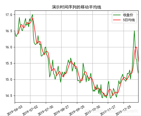
8 df['Close'].plot(color="green",label='收盘价')
9 df['Close'].rolling(window=5).mean().plot(color="red",label='5日均线')
10 plt.legend(loc='best') # 绘制图例
11 ax.grid(True) # 带网格线
12 plt.title("演示时间序列的移动平均线")
13 plt.rcParams['font.sans-serif']=['SimHei']
14 plt.setp(plt.gca().get_xticklabels(), rotation=30)
15 plt.show()In this example, the matplotlib visualization control is used. Specifically, after the data is obtained from the csv file through the code in line 5, the plot method in line 8 is used to connect the points of the daily closing price in the df object in turn, thereby A broken line describing the "closing price" is drawn.
In the 9th line of the rolling method, the window of the mobile analysis is specified by the window parameter to be 5 days, and combined with the mean method, a 5-day moving average line based on the closing price is drawn. Please note that when drawing two polylines on the 8th and 9th rows, the legend is set by the label parameter, so in the 10th row afterwards, the legend effect can be set by the legend method.
Also worth noting is the visualization details. In line 11, the grid lines are set by the grid method, the Chinese title is set by the code in lines 12 and 13, and the x-axis coordinate text is specified in line 14. The label needs to be rotated 30 degrees.
Run the above code, you can see the effect as shown in the figure below. If you compare the closing price and the moving average, you will find that the latter is much smoother. From this, everyone can feel that the moving average based on time series can eliminate random fluctuations to a certain extent, and can more effectively display the fluctuations of sample data. trend.
2 Autocorrelation analysis of closing price based on time series
Correlation refers to whether there is a correlation between two sets of data, that is, whether changes in one set of data will affect another set of data. The autocorrelation refers to whether there is a correlation between variables at two different points in the same time series.
Here is another example of stock closing prices. In this scenario, autocorrelation refers to whether there is a correlation between the closing prices of two trading days. Like correlation, autocorrelation is also represented by a number from -1 to 1, where 0 also means irrelevance, 1 also means complete correlation, and -1 means complete reverse correlation. What is the statistical significance of autocorrelation?
- If two similar values are not correlated in the time series, that is, the correlation coefficient is 0, it means that there is no correlation between the points on the time series. Then there is no need to observe the law to predict future data. Specifically in the case of the stock closing price, if there is no correlation between the closing price of the current trading day and the closing price of the previous trading day, then there is no need to analyze the closing price of the previous trading day to predict the closing price of the future trading day. In other words, only when there is a correlation between the values of different points in the time series, it is necessary to analyze the laws of the past to calculate the future value.
- The autocorrelation coefficient of a stationary series should quickly converge (or decay) to zero. A stationary series means that the changing law of the data in the time series will basically remain unchanged, so that the law analyzed from the past data can be used to calculate the future value. In the case of the stock closing price, the closing price of the day can be correlated with the closing price in the next week, but in a stationary sequence, the closing price of the day and the future long-term (assuming 50 days) day closing price are not correlated. On the contrary, it means that changes in the closing price of any day will affect a long period of time, accumulating over time, so when predicting the closing price of a certain day in the future, you must also consider the law of too much influence in the past for a long time, then the law of the time series will change. Is too complicated, which will lead to unpredictability,
That is to say, for a time series, only when the data in the similar time in the series are correlated, and the data with a long interval are not correlated, the series has the significance of being statistically analyzed. The autocorrelation algorithm is not simple, but the autocorrelation in the time series can be calculated by the method encapsulated in the statsmodels library.
Before using this library, you still need to install it through the pip3 install statsmodels command. The author installed the latest version 0.11.1. After installation, in order to be able to use it correctly, you also need to install the mkl and scipy libraries. In the following AcfDemo.py example, we will use the case of stock closing prices to let everyone intuitively feel the autocorrelation in the time series.
1	#coding=utf-8
2	import pandas as pd
3	import statsmodels.api as stats
4	filename='D:\\work\\data\\ch9\\6007852019-06-012020-01-31.csv'
5	df = pd.read_csv(filename,encoding='gbk',index_col=0)
6	stats.graphics.tsa.plot_acf(df['Close'],use_vlines=True,lags=50, title = 'ACF Demo')
In the third line, the statsmodels library for calculating the autocorrelation coefficient is introduced. In the fifth line, the data of the stock closing price is read from the specified file, and in the sixth line, the stats.graphics.tsa.plot_acf method is used To calculate and draw a graph of the correlation coefficient of the closing price.
The use_vlines parameter of this method indicates whether to set the connection between the point and the x-axis. The value here is True, which indicates that it needs to be set. The lags parameter indicates the autocorrelation coefficient from the data of the day to the next 50 days, and the title parameter indicates the chart title. Run this example, you can see the effect as shown in the figure below.
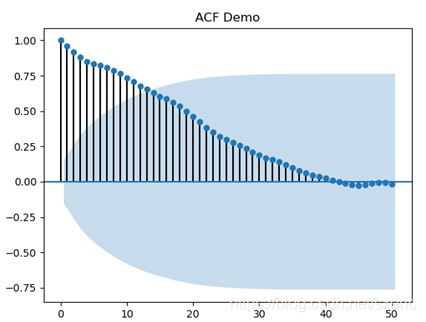
As can be seen from the above figure, the scale of the x-axis ranges from 0 to 50, which matches the value of the lags parameter, and the scale of the y-axis ranges from -1 to 1, which represents the coefficient of autocorrelation. Further analysis, the following statistical significance can be seen from the above figure.
- The autocorrelation coefficient with a value of 0 on the x-axis is 1, which means that the data of the day is completely correlated with itself.
- Some autocorrelation coefficients on the x-axis close to 0 are very close to 1. For example, the autocorrelation coefficients of the 13th day and the 14th day and the 15th day are relatively small, which shows that the closing price of the day has a certain impact on the future closing price in the near future. .
- As the value of the x-axis becomes larger, the autocorrelation coefficient gradually decays, and when it is close to 40, it basically decays to 0. This shows that the change in the closing price of a certain day will not have an impact on the long-term future data, which in turn shows that the series is stable.
- In addition to the points and lines describing the autocorrelation coefficient, there is also a blue area describing the 95% confidence interval. From the figure, the autocorrelation coefficient for 13 days is about 0.7, and it falls within the blue area. This means that the autocorrelation coefficients of the data on the 1st and 13th days have a 95% confidence level, while the 95% confidence level has not been reached before. The reason for not reaching 95% credibility before is that the data in this scenario is from June 1, 2019. In the actual scenario, the closing price of the trading day will be affected by the previous data, but the data here is only from Since June 1st, the association with the previous data has been lost, resulting in a decrease in credibility.
- Observe the autocorrelation coefficients on the 13th, 14th, and 15th days that fall within the 95% confidence interval. The relative difference between them is not big.
The conclusion drawn from the above is that the closing price of the stock based on the time series has a certain degree of autocorrelation in a relatively short period, and the credibility reaches or exceeds 95%, and the series is stable. Therefore, it is necessary to analyze the closing price sequence of the stock, and the law obtained from it can predict the future trend to a certain extent. For other time series, the autocorrelation can also be analyzed in this step, and corresponding conclusions can be drawn in this way.
3 Analysis of partial autocorrelation of closing price based on time series
It can be seen from the above example that if the data based on the time series has autocorrelation, then this autocorrelation is very likely to be passed, that is, the data of the nth day is affected by the data of the n-1th day, and the nth -1 day's data is affected by n-2 days, and so on, the nth day's data may be affected by the combined effects of several previous data. Specific to the case of the closing price, that is, the closing price of the day will not only be affected by the previous trading day, but also indirectly by several previous trading days.
In some statistical scenarios, the indirect influence of earlier data needs to be eliminated, and only the direct influence of previous data on the current data is measured. This can use the "partial autocorrelation coefficient".
The calculation process of "partial autocorrelation coefficient" is quite complicated. According to the algorithm, the "indirect influence" contained in the autocorrelation coefficient has been eliminated. In practical applications, it can also be achieved by calling the relevant methods in the statsmodels library, in the following PacfDemo In the .py example, the method of calculating and plotting partial autocorrelation coefficients will be demonstrated.
1	#coding=utf-8
2	import pandas as pd
3	import statsmodels.api as stats
4	filename='D:\\work\\data\\ch9\\6007852019-06-012020-01-31.csv'
5	df = pd.read_csv(filename,encoding='gbk',index_col=0)
6	stats.graphics.tsa.plot_pacf(df['Close'],use_vlines=True,lags=50, title = 'PACF Demo')
This example is very similar to the previous example of seeking autocorrelation. The difference is that in line 6, the plot_pacf method is called to calculate and plot the partial autocorrelation coefficient. Run this example and you can see the effect as shown in the figure below.

Excluding the first two data, most of the data fall within the blue 95% confidence interval, and the partial autocorrelation coefficient is between -0.15 and 0.15. This shows that if you exclude the impact of the data on the earlier trading day and simply look at the closing prices of the day and the next trading day, their correlation is about 0.15. This conclusion has 95% credibility. After integrating the autocorrelation coefficient, it shows that when predicting the future closing price, we should not only consider the impact of the previous trading day, but also introduce the closing price of the earlier trading day as a reference factor.
4 Use the heat map to analyze the correlation of different time series
Previously, autocorrelation coefficients and partial autocorrelation coefficients were used to measure the impact of data before and after a single time series. In application, the correlation of different time series will also be quantitatively analyzed.
For example, when formulating a stock trading strategy, the correlation between the closing prices of different stocks will be quantitatively calculated. If their positive correlation is strong, it means that their trend patterns are very similar. In this section, we will show you the correlation between the closing prices of stocks as shown in the following table in the form of a heat map.
Table Analyze the list of relevant stock information
| Stock code |
Stock name |
Owned sector |
| 603005 |
Jingfang Technology |
semiconductor |
| 600360 |
China Microelectronics |
semiconductor |
| 600640 |
Haobai Holdings |
Internet media |
In the following example of CompareCorrByHeatMap.py, the data of the specified stock will be captured from the web interface first, the correlation between the stocks will be calculated on this basis, and the effect of the correlation between different time series will be visually displayed in the form of a heat map.
1	#coding=utf-8
2	import pandas as pd
3	import matplotlib.pyplot as plt
4	import pandas_datareader
5	# 603005 晶方科技 半导体
6	# 600360 华微电子 半导体
7	# 600640 号百控股 互联网传媒
8	stockCodes = ['603005', '600360', '600640']
9	start='2019-12-01'
10	end='2020-01-31'
11	stockCloseDF = pd.DataFrame()
12	for code in stockCodes:
13	    thisClose = pandas_datareader.get_data_yahoo(code + '.ss', start, end)
14	    stockCloseDF[code] = thisClose['Close'].values
15	#print(stockCloseDF) #可以观察结果
16	fig = plt.figure()
17	ax = fig.add_subplot(111)
18	ax.set_xticklabels(stockCodes)
19	ax.set_xticks(range(len(stockCodes)))
20	ax.set_yticklabels(stockCodes)
21	ax.set_yticks(range(len(stockCodes)))
22	im = ax.imshow(stockCloseDF.corr(), cmap=plt.cm.hot_r)
23	# 添加颜色刻度条
24	plt.colorbar(im)
25	# 添加中文标题
26	plt.rcParams['font.sans-serif']=['SimHei']
27	plt.title("用热力图观察股票间的相关性")
28	plt.xlabel('股票代码')
29	plt.ylabel('股票代码')
30	plt.show()
In the stockCodes variable on line 8, the stock codes to be analyzed are defined. Please refer to the comments on lines 5 to 7 for the specific information of these stocks. At the same time, define the codes to be analyzed in the codes on lines 9 and 10. The start and end date of the stock.
Then in the for loop from line 12 to line 14, traverse the stock codes in turn, and get the corresponding data from the network interface, and put the closing prices of the three stocks into the stockCloseDF object of the DataFrame type in the 14th line. Now that the data preparation is completed, you can also open the comment on line 15 and observe the result through the print statement.
After the data is obtained, in the code on lines 22 and 24, the correlation between each strand will be calculated two by one, and the heat map will be drawn, and the color scale bar of the legend nature will be displayed on the right. Run this example, you can see the effect as shown in the figure below.
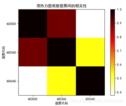
As you can see from the figure above, the x-axis and y-axis scales are both stock codes. After pairwise comparison, their correlations are both 1, while 603005 (Jingfang Technology) and 600360 (Huawei Electronics) are both semiconductors. The correlation between them is relatively high, and 600640 (Haobai Holdings) belongs to the Internet media sector, so its correlation with the other two stocks is very low.
This article is from a self-written book: Python crawler, data analysis and visualization: detailed tool explanation and case combat, https://item.jd.com/10023983398756.html

Please pay attention to my official account: make progress together and make money together. In this official account, there will be many wonderful articles.
