The convolutional neural network mentioned in the previous article recognizes handwritten digits with a recognition rate of 99.15%. For comparison, let’s compare the linear model LN, single neural network SN, and deep neural network DNN to simulate the same test data to see To the power of convolutional neural networks.
The test results are as follows:
| Model name | Correct rate |
|---|---|
| Convolutional Neural Network | 99.15% |
| Linear model | 31.32% |
| Single neuron model | 92.49% |
| Deep neural network | 96.97% |
Conclusion and analysis: Convolutional neural networks are unmatched in the field of image processing.
| Model name | Analyze the reasons |
|---|---|
| Linear model | Only linear problems can be divided, non-linear problems can't do anything |
| Single neuron model | Can handle nonlinear problems, the structure is too simple, and the extraction of features is not enough |
| Deep neural network | A lot of features can be extracted, and it is precisely because all the details are extracted, which leads to over-fitting, and the result is not good. Too buckle details |
| Convolutional Neural Network | It can be understood as a sparse deep neural network. Operations such as convolution and pooling actually select local image information to extract features, thereby reducing complexity and avoiding over-fitting. Multiple convolution kernels extract features from multiple aspects, and the features are very comprehensive, but I don’t care about every detail |
Article Directory
Implement various models with TensorFlow2
Based on the convolutional neural network in the previous article, you can get a variety of models with a little change.
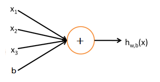
1. Linear model
The linear model is what we often say y = k*x + b. It can only represent a linear division. The model is as follows:
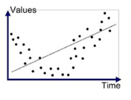
Only such a curve can be fitted:
tf Implementation method: Use a fully connected Dense, and use a linear function for the activation function.
The code is as follows: see the previous article for testData in from testData import *. testData
import numpy as np
import tensorflow as tf
from testData import *
import time

class LINE(tf.keras.Model):
    def __init__(self):
        super().__init__()
        self.line = tf.keras.layers.Dense(units=10,activation=tf.keras.activations.linear)  #一个神经元的全连接网络,激活函数是线性的
        self.flatten = tf.keras.layers.Reshape(target_shape=(28*28,))  #把二维的矩阵展平为1维

    def call(self,inputs):
        x = self.flatten(inputs)  #拉平成一个大的一维向量
        x = self.line(x)   #经过第一个全连接层
        output = x
        return output

#主控程序,调用数据并训练模型
#定义超参数
num_epochs = 5  #每个元素重复训练的次数
batch_size = 50
learning_rate = 0.001

print('now begin the train, time is ')
print(time.strftime('%Y-%m-%d %H:%M:%S',time.localtime()))
model = LINE()
data_loader = MNISTLoader()
optimier = tf.keras.optimizers.Adam(learning_rate=learning_rate)

num_batches = int(data_loader.num_train_data//batch_size*num_epochs)
for batch_index in range(num_batches):
    X,y = data_loader.get_batch(batch_size)
    with tf.GradientTape() as tape:
        y_pred = model(X)
        loss = tf.keras.losses.sparse_categorical_crossentropy(y_true=y,y_pred=y_pred)
        loss = tf.reduce_sum(loss)
        print("batch %d: loss %f"%(batch_index,loss.numpy()))
    grads = tape.gradient(loss,model.variables)
    optimier.apply_gradients(grads_and_vars=zip(grads,model.variables))

print('now end the train, time is ')
print(time.strftime('%Y-%m-%d %H:%M:%S', time.localtime()))
#模型的评估
sparse_categorical_accuracy = tf.keras.metrics.SparseCategoricalAccuracy()
num_batches_test = int(data_loader.num_test_data//batch_size)  #把测试数据拆分成多批次,每个批次50张图片
for batch_index in range(num_batches_test):
    start_index,end_index = batch_index*batch_size,(batch_index+1)*batch_size
    y_pred = model.predict(data_loader.test_data[start_index:end_index])
    sparse_categorical_accuracy.update_state(
        y_true = data_loader.test_label[start_index:end_index],
        y_pred=y_pred
    )
print('test accuracy: %f'%sparse_categorical_accuracy.result())
print('now end the test, time is ')
print(time.strftime('%Y-%m-%d %H:%M:%S',time.localtime()))
As a result, the correct rate is only 31.32%
2. Single neuron model
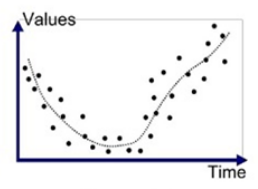
The single neuron model is based on the
linear model , and the activation function is added to the finishing touch. With it, the linear model can become a non-linear model, which can fit more complex scenes.
As follows:
The relationship between the single neuron model and the linear model is as follows:

TensorFlow2 realizes the single neuron model, which is based on the linear model, plus activation functions, such as softmax and relu functions. Common activation functions are introduced as follows: the activation function
code is as follows: from testData import * testData in the previous article. testData
import numpy as np
import tensorflow as tf
from testData import *
import time

class SNN(tf.keras.Model):
    def __init__(self):
        super().__init__()
        self.line = tf.keras.layers.Dense(units=10,activation=tf.nn.softmax)  #一个神经元的全连接网络,激活函数是非线性的
        self.flatten = tf.keras.layers.Reshape(target_shape=(28*28,))  #把二维的矩阵展平为1维

    def call(self,inputs):
        x = self.flatten(inputs)  #拉平成一个大的一维向量
        x = self.line(x)   #经过第一个全连接层
        output = x
        return output

#主控程序,调用数据并训练模型
#定义超参数
num_epochs = 5  #每个元素重复训练的次数
batch_size = 50
learning_rate = 0.001

print('now begin the train, time is ')
print(time.strftime('%Y-%m-%d %H:%M:%S',time.localtime()))
model = SNN()
data_loader = MNISTLoader()
optimier = tf.keras.optimizers.Adam(learning_rate=learning_rate)

num_batches = int(data_loader.num_train_data//batch_size*num_epochs)
for batch_index in range(num_batches):
    X,y = data_loader.get_batch(batch_size)
    with tf.GradientTape() as tape:
        y_pred = model(X)
        loss = tf.keras.losses.sparse_categorical_crossentropy(y_true=y,y_pred=y_pred)
        loss = tf.reduce_sum(loss)
        print("batch %d: loss %f"%(batch_index,loss.numpy()))
    grads = tape.gradient(loss,model.variables)
    optimier.apply_gradients(grads_and_vars=zip(grads,model.variables))

print('now end the train, time is ')
print(time.strftime('%Y-%m-%d %H:%M:%S', time.localtime()))
#模型的评估
sparse_categorical_accuracy = tf.keras.metrics.SparseCategoricalAccuracy()
num_batches_test = int(data_loader.num_test_data//batch_size)  #把测试数据拆分成多批次,每个批次50张图片
for batch_index in range(num_batches_test):
    start_index,end_index = batch_index*batch_size,(batch_index+1)*batch_size
    y_pred = model.predict(data_loader.test_data[start_index:end_index])
    sparse_categorical_accuracy.update_state(
        y_true = data_loader.test_label[start_index:end_index],
        y_pred=y_pred
    )
print('test accuracy: %f'%sparse_categorical_accuracy.result())
print('now end the test, time is ')
print(time.strftime('%Y-%m-%d %H:%M:%S',time.localtime()))
Three, deep neural network
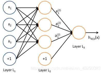
A deep neural network can be understood as a stack of single neural networks. Some dimensionality reduction and other processing may be performed in the middle. The activation function of each layer can be different, so there are many combinations, and each layer can choose full connection, partial connection, and random connection. Wait, a lot of combinations.
The structure is as follows:
The code is as follows (do it yourself to add 3 fully connected layers), see the previous article for testData in from testData import *. testData
import numpy as np
import tensorflow as tf
from testData import *
import time

class DNN(tf.keras.Model):
    def __init__(self):
        super().__init__()
        self.dense1 = tf.keras.layers.Dense(units=50, activation=tf.nn.relu)  # 一个神经元的全连接网络,激活函数是非线性的
        self.dense2 = tf.keras.layers.Dense(units=100,activation=tf.nn.relu)  #一个神经元的全连接网络,激活函数是非线性的
        self.flatten = tf.keras.layers.Reshape(target_shape=(28*28,))  #把二维的矩阵展平为1维
        self.dense3 = tf.keras.layers.Dense(units=10, activation=tf.nn.softmax)  # 一个神经元的全连接网络,激活函数是非线性的

    def call(self,inputs):
        x = self.flatten(inputs)  #拉平成一个大的一维向量
        x = self.dense1(x)   #经过第一个全连接层
        x = self.dense2(x)  # 经过第2个全连接层
        x = self.dense3(x)  # 经过第3个全连接层
        output = x
        return output

#主控程序,调用数据并训练模型
#定义超参数
num_epochs = 5  #每个元素重复训练的次数
batch_size = 50
learning_rate = 0.001

print('now begin the train, time is ')
print(time.strftime('%Y-%m-%d %H:%M:%S',time.localtime()))
model = DNN()
data_loader = MNISTLoader()
optimier = tf.keras.optimizers.Adam(learning_rate=learning_rate)

num_batches = int(data_loader.num_train_data//batch_size*num_epochs)
for batch_index in range(num_batches):
    X,y = data_loader.get_batch(batch_size)
    with tf.GradientTape() as tape:
        y_pred = model(X)
        loss = tf.keras.losses.sparse_categorical_crossentropy(y_true=y,y_pred=y_pred)
        loss = tf.reduce_sum(loss)
        print("batch %d: loss %f"%(batch_index,loss.numpy()))
    grads = tape.gradient(loss,model.variables)
    optimier.apply_gradients(grads_and_vars=zip(grads,model.variables))

print('now end the train, time is ')
print(time.strftime('%Y-%m-%d %H:%M:%S', time.localtime()))
#模型的评估
sparse_categorical_accuracy = tf.keras.metrics.SparseCategoricalAccuracy()
num_batches_test = int(data_loader.num_test_data//batch_size)  #把测试数据拆分成多批次,每个批次50张图片
for batch_index in range(num_batches_test):
    start_index,end_index = batch_index*batch_size,(batch_index+1)*batch_size
    y_pred = model.predict(data_loader.test_data[start_index:end_index])
    sparse_categorical_accuracy.update_state(
        y_true = data_loader.test_label[start_index:end_index],
        y_pred=y_pred
    )
print('test accuracy: %f'%sparse_categorical_accuracy.result())
print('now end the test, time is ')
print(time.strftime('%Y-%m-%d %H:%M:%S',time.localtime()))
Model summary
By comparing the linear model and the single neuron model with the activation function, it can be seen that the activation function is simply a magic trick, which improves the accuracy a lot at once.
In the field of image recognition, the accuracy of multiple neural networks is not as accurate as that of convolutional neural networks, which may be caused by overfitting.