EXCEL data analysis (1)

function

Statistical analysis functions, text processing functions, numerical calculation functions, logical judgment functions, date calculation functions, matching search functions.

1. Statistical analysis functions
   count, counta, countblack, countif, countifs, sum, sumif, average, averageif, averageifs, max, dmax, min, dmin, large, small, rank, sumproduct
   
   ① The count function
   calculates the number of cells containing numbers in the area number.
   =COUNT(G2:G9)
   ②counta function
   Calculates the number of non-empty cells in the area.
   =COUNTA(D2:D9)
   ③countblack function
   Calculates the number of empty cells in a certain area.
   =COUNTBLANK(D2:D9)
   ④countif function Counts
   the number of cells that meet a certain condition.
   =COUNTIF(C:C,I2)
   ⑤countifs function
   applies conditions to cells that span multiple areas, and then counts the number of cells that meet all conditions.
   =COUNTIFS(B:B,"Shanghai",C:C,"F")

⑥sum function
Calculates the sum of all values ​​in the cell area.
=SUM(G2:G9)
⑦sumif function
sums the cells that meet the conditions (single condition summation).
=SUMIF(C:C,"M",G:G)
⑧sumifs function
sums the cells specified by a group of given conditions (summation of multiple conditions).
=SUMIFS(G:G,B:B,"Guangzhou",C:C,"F")

⑨average function
returns the average value in a set of values.
=AVERAGE(G2:G9)
⑩averageif function
returns the average value (arithmetic average) of all cells that meet a single condition.
=AVERAGEIF(C:C,"F",G:G)
①The averageifs function
returns the average value (arithmetic average) of all cells that meet multiple conditions.
=AVERAGEIFS(G:G,B:B,"Shanghai",C:C,"M")

②The max function
returns the maximum value in a set of values.
=MAX(G2:G9)
③ The dmax function
returns the largest number in the record field (column) that meets the specified conditions in the list or database.
=DMAX($A $1:$G$9,$ G$1,I1:J2)④mIn-functionnumberreturnsback\; toaset\; ofvaluesinthemostsmallvalue.=MIN(G2:G.\; 9)⑤DmIn-functionnumberreturnsback\; to\; thecolumnslistorthe\; number\; ofdatadatabaseinfullfootfingerspecifiedstripmemberisreferred\; torecordwordsegment(column)inthemosta\; smallnumber\; ofwords.=DMIN($A$1:$G$9,$G$1,I1:J2)

⑥The large function
returns the k-th largest value in the data set.
=LARGE(G2:G9,2)
⑦small function
returns the k-th smallest value in the data set.
=SMALL(G2:G9,2)

⑧The rank function
returns the sort position of a number in a set of numbers. If order is 0 or omitted, it will be sorted in descending order by default.
=RANK(G2,$G $2:$G$9,0)

⑨sumproduct function
In the given groups of arrays, multiply the corresponding elements between the arrays and return the sum of the products.
=SUMPRODUCT(C2:C8,D2:D8)

2. Text processing functions
   len, lenb, left, leftb, right, rightb, mid, midb, upper, lower, search, searchb, find, findb, replace, replaceb, substitute, substituteb, trim, concatenate, exact
   ① The len function
   returns a text string The number of characters in.
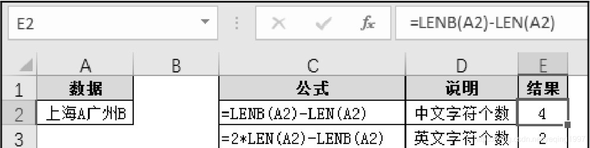
   The LEN function counts the number of characters, which is equivalent to 1 Chinese characters + 1 English characters (or numbers).
   ②The lenb function
   returns the number of bytes used to represent characters in a text string.
   The LENB function counts the number of bytes, which is equivalent to 2 Chinese characters + 1 English characters (or numbers).
   

③The left function
LEFT returns the specified number of characters starting from the first character of the text string.
=LEFT(A2,3)
④The right function
RIGHT returns the last one or more characters in the text string according to the specified number of characters.
=RIGHT(A2,3)

⑤The mid function
MID returns a specific number of characters from the specified position in the text string, and the number is specified by the user.
=MID(A2,4,2)

⑥ The upper function
UPPER converts the text into uppercase letters.
=UPPER(A2)
⑦The lower function
LOWER converts the text into lowercase letters.
=LOWER(A2)

⑧find function is
used to locate the first text string in the second text string, and return the value of the starting position of the first text string, which starts from the first character of the second text string.
start_num is optional. Specify the position of the character to start the search. If omitted, it defaults to 1. Functions are case sensitive.
=FIND("Data",A2,1)

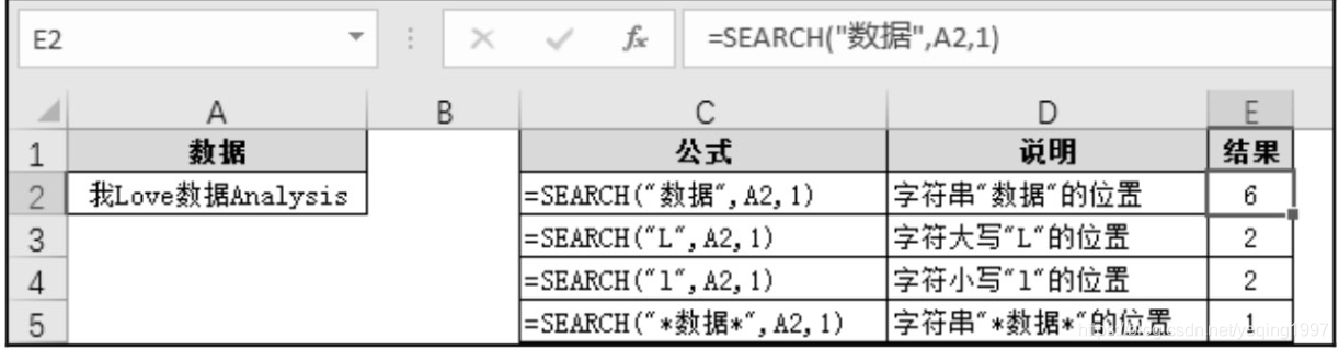
⑨Search function
SEARCH function can find the first text string in the second text string, and returns the number of the starting position of the first text string, which is from the first character of the second text string Count.
The wildcard "*" matches any character, so " data " matches the entire string "I Love Data Analysis". The returned result is to search from the first character. The position of the string "My Love Data Analysis" in the string "My Love Data Analysis" is the position of the first character "I" of the search string, and finally 1 is returned. .

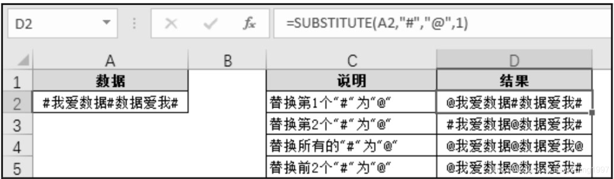
⑩The substitute function is
used to replace the specified text in a text string, replacing old_text with new_text.

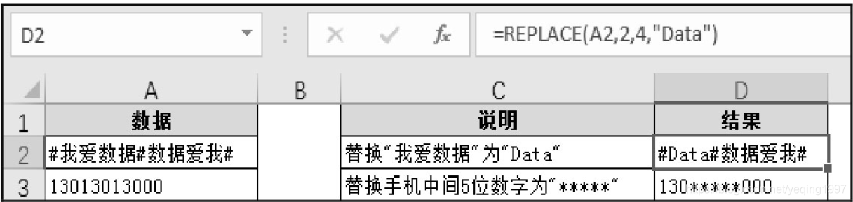
①Replace function
According to the specified number of characters, REPLACE replaces part of the text string with a different text string.
The difference between the REPLACE function and the SUBSTITUTE function: The REPLACE function specifies the starting position and character length for replacement; and the SUBSTITUTE function replaces the given original string with a new string.
The REPLACE function also has similarities with the MID function mentioned above: the MID function is intercepted according to the starting position and the character length; and the REPLACE function, in addition to intercepting, also replaces the intercepted string.

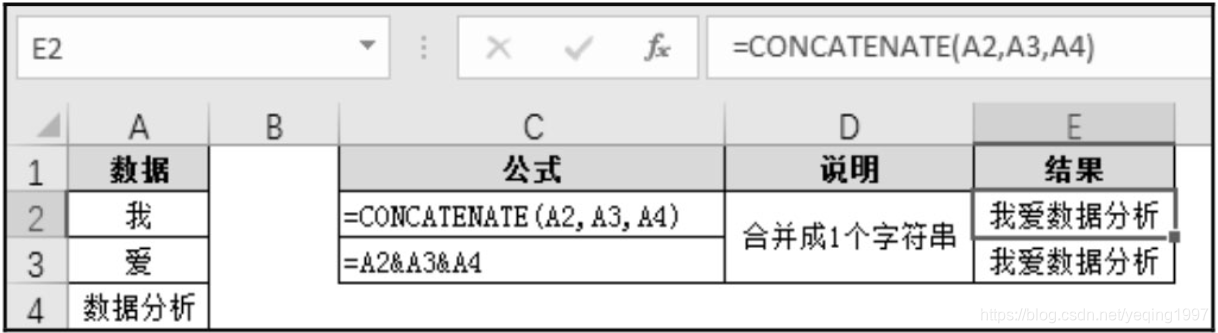
②The concatenate function
connects two or more strings into one string.

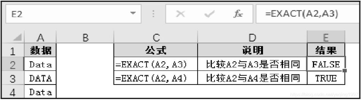
③exact function

④trim function
Remove all spaces in the text except for a single space between words.

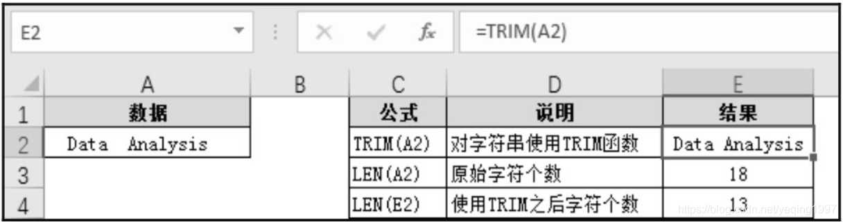
All the spaces at the front and back ends of the string are removed.
One space between words in the string is reserved.

3. Numerical calculation functions
   Random value generation rand, randbetween functions, abs, mod, power, product functions for mathematical operations, ceiling, floor, round, roundup, rounddown, trunc functions, etc. for rounding, rounding up and down.
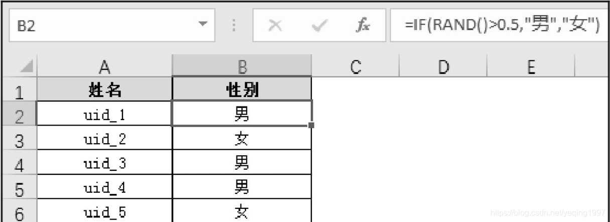
   ① The rand function
   returns an evenly distributed random real number that is greater than or equal to 0 and less than 1, and a new random real number is returned every time the worksheet is calculated.
   
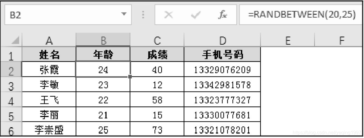
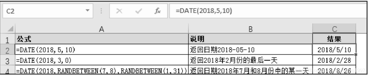
   ②The randbetween function
   returns a random integer between two specified numbers. A new random integer will be returned every time the worksheet is calculated.
   Enter the formula "=RANDBETWEEN(20,25)" in cell B2, and then drag down to copy the formula.
   Enter the formula "=RANDBETWEEN(0,100)" in cell C2, and then drag down to copy the formula.
   Enter the formula "="133" &RANDBETWEEN(10000000, 99999999)" in cell D2, and then drag down to copy the formula.
   
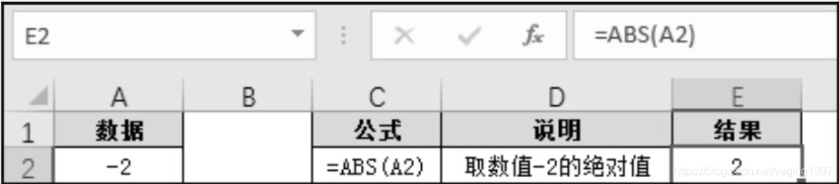
   ③abs function
   returns the absolute value of a number.
   
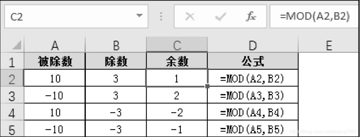
   ④mod function
   returns the remainder of the division of two numbers. The sign of the returned result is the same as the divisor.
   
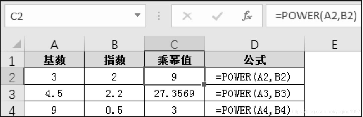
   ⑤The
   power function returns the result of number power.
   
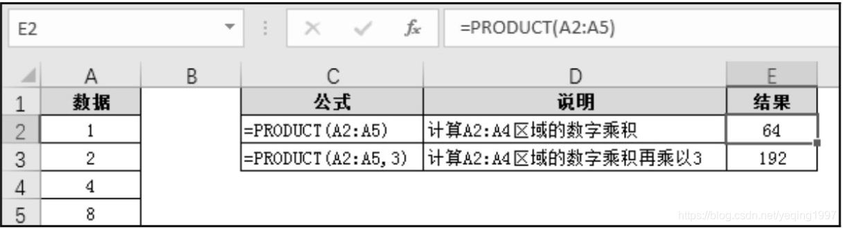
   ⑥The product function
   multiplies the numbers given in the parameter form and returns the product.
   
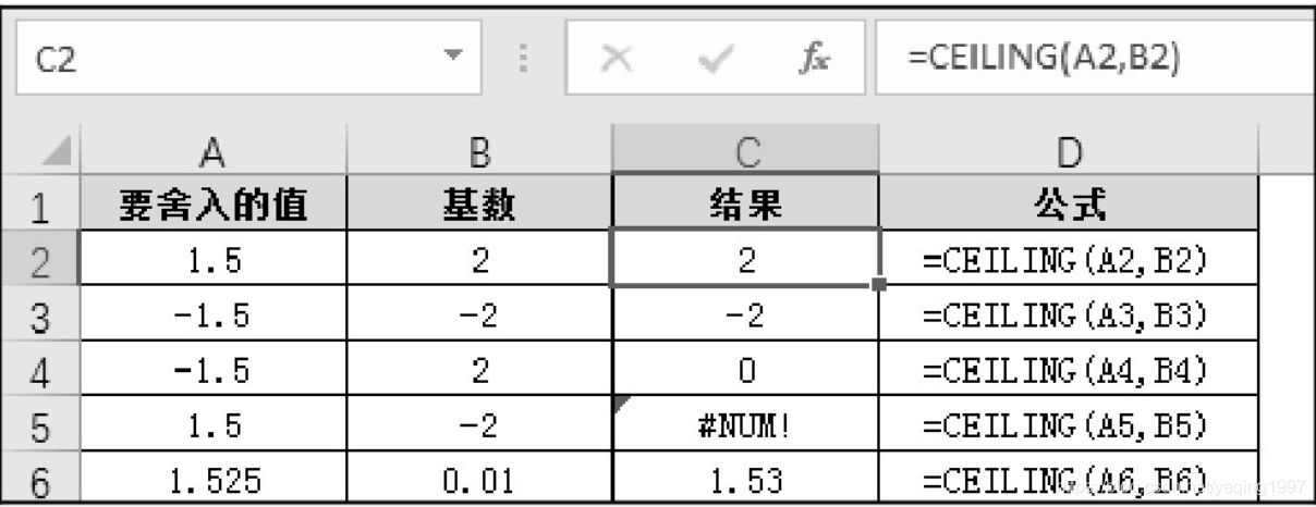
   ⑦ceiling function
   returns the parameter number to be rounded up (in the direction of increasing absolute value) to the nearest multiple of the specified base.
   
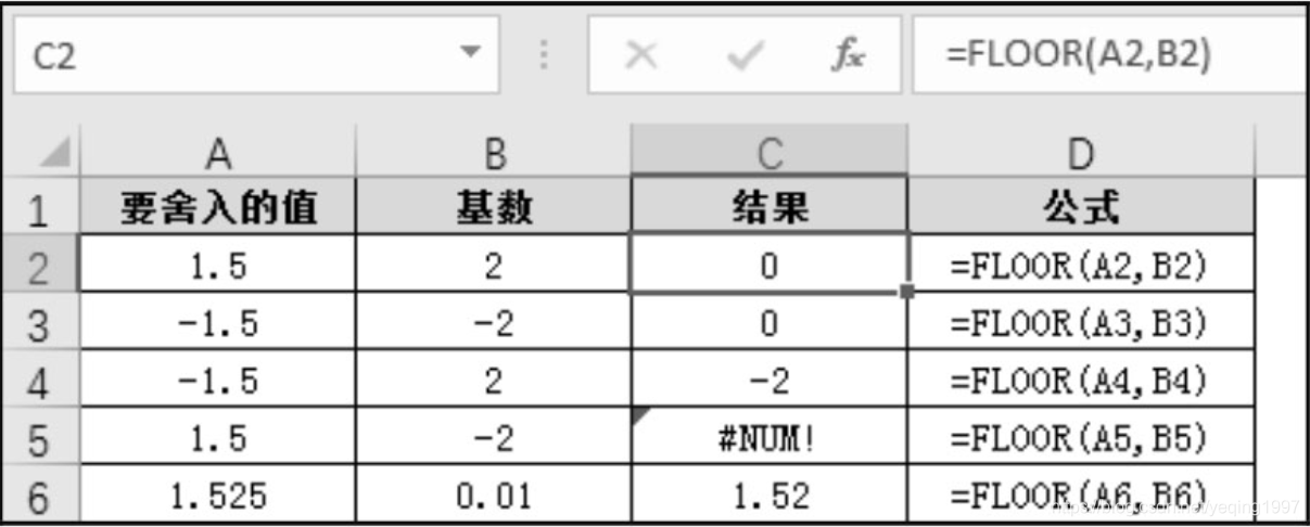
   ⑧The floor function
   rounds the parameter number down (in the direction of decreasing absolute value) to the nearest multiple of the specified base.
   
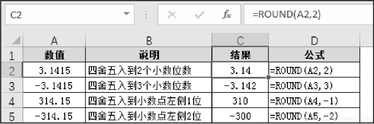
   ⑨round function
   ROUND function rounds the number to the specified number of digits.
   
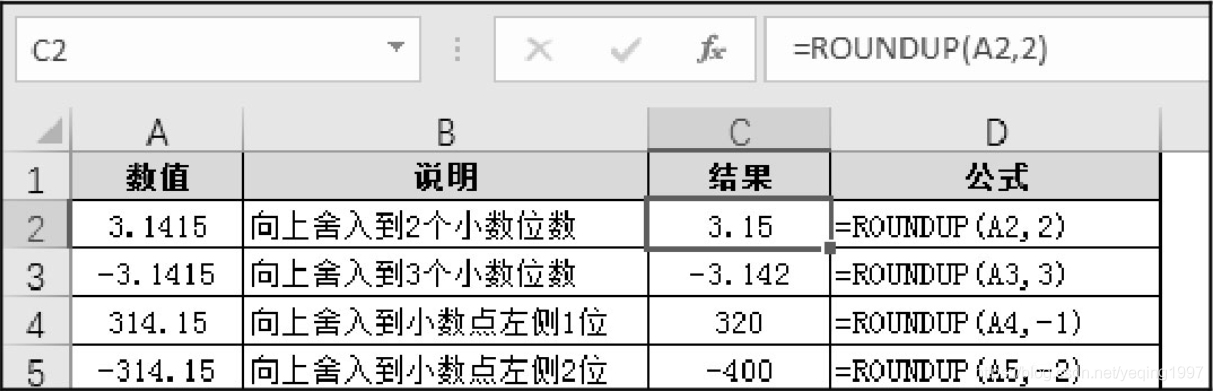
   ⑩roundup function
   Rounds up the number away from the value 0.
   
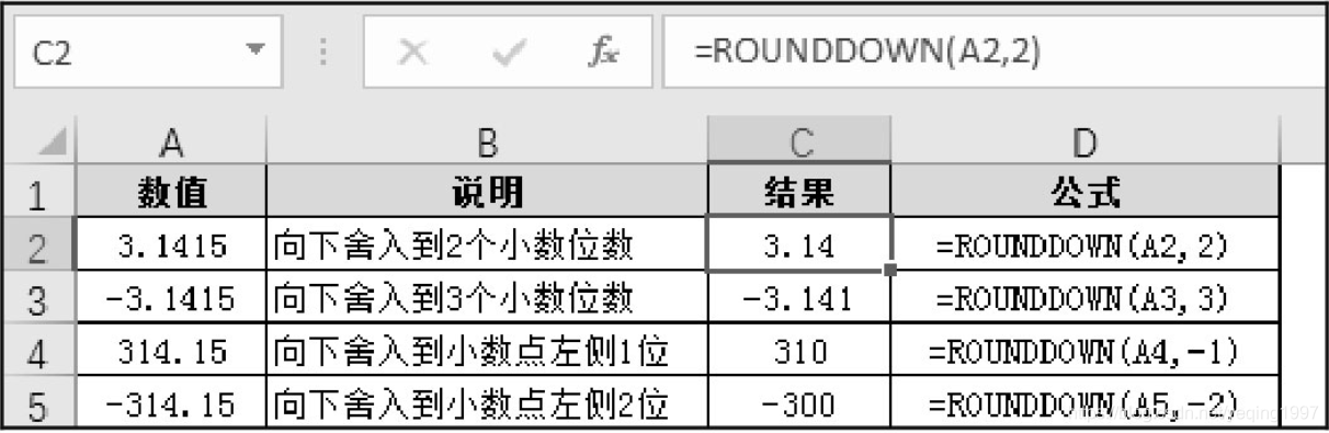
   ①The rounddown function
   rounds down the number towards the value 0.
   
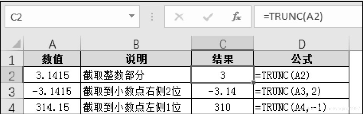
   ②The trunc function
   intercepts the number and returns an integer.
   
4. Logical judgment functions
   Common logical judgment functions include and, or, not, if, iferror, is series (including iserror, istext, isnumber, etc.). The IF function is often used for nested judgments of multiple conditions, for example, to judge the sales commission coefficient based on the salesperson's performance range. In addition, AND and OR functions can be used to check and judge multiple conditions.
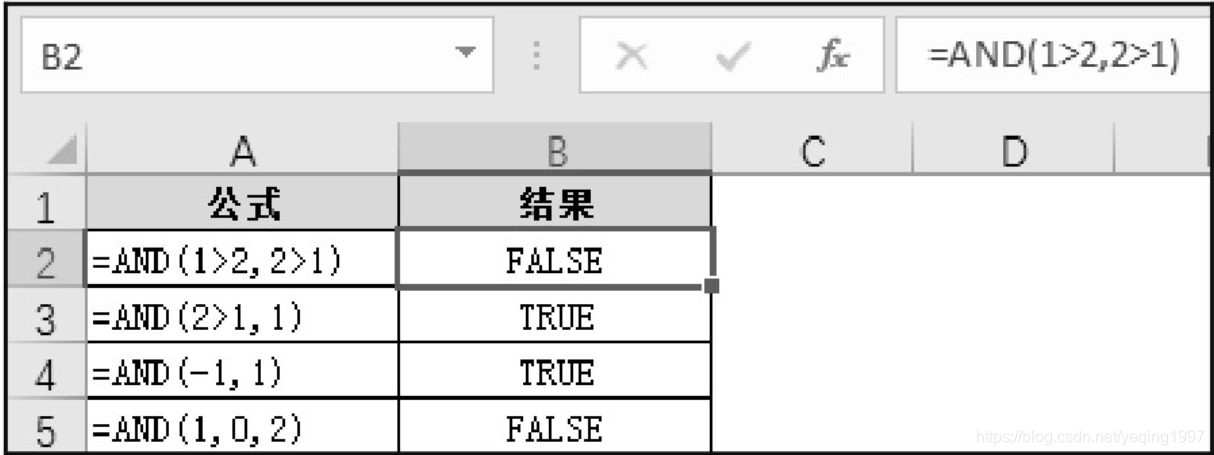
   ①and function
   checks whether all the parameters are TRUE, if all the parameter values ​​are TRUE, it returns TRUE.
   
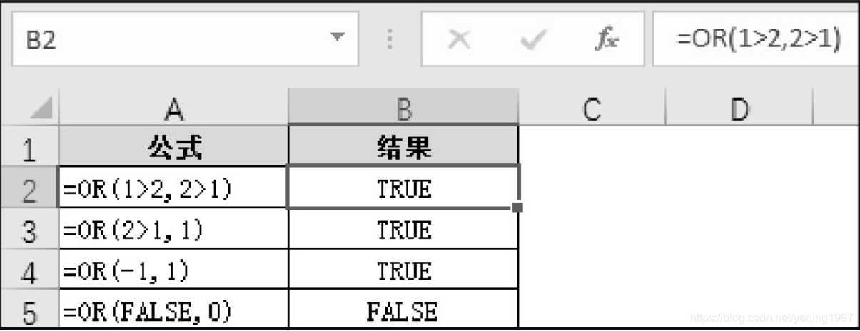
   ②or function
   If any parameter is TRUE, it returns TRUE; only when all the parameter values ​​are FALSE will it return FALSE.
   
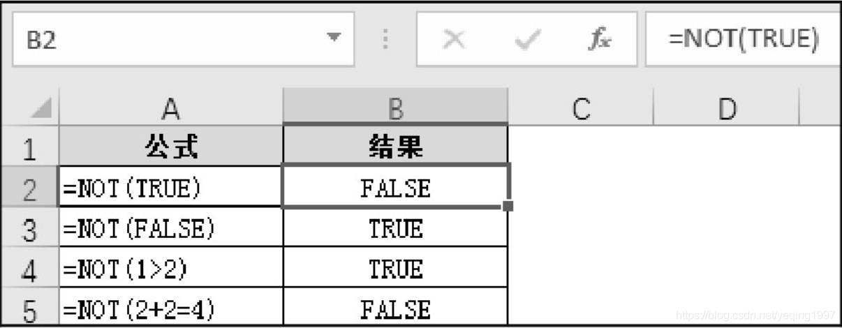
   ③not function negates
   the logical value of the parameter: returns FALSE when the parameter is TRUE, and returns TRUE when the parameter is FALSE.
   

④if function
Judge whether a certain condition is met, return a value if it is met, and return another value if it is not met.
Method 1: Input the formula "=IF(D3＜60,"Failed",IF(D3＜85,"Pass","Excellent"))" in cell E3, and then drag down to copy the formula.
Method 2: Input the formula "=IF(D3＞=85,"Excellent",IF(D3＞=60,"Pass","Fail")) in cell F3, then drag down to copy the formula, the result As shown in Figure 2-67.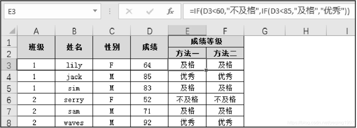
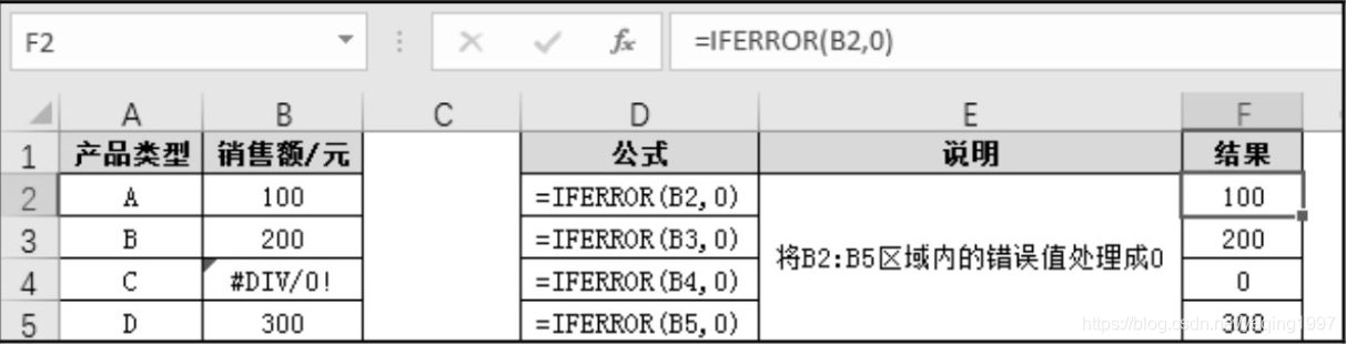
⑤iferror function
If the expression is an error, it returns value_if_error, otherwise it returns the value of the expression itself.

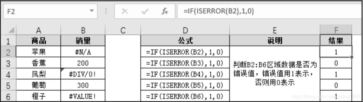
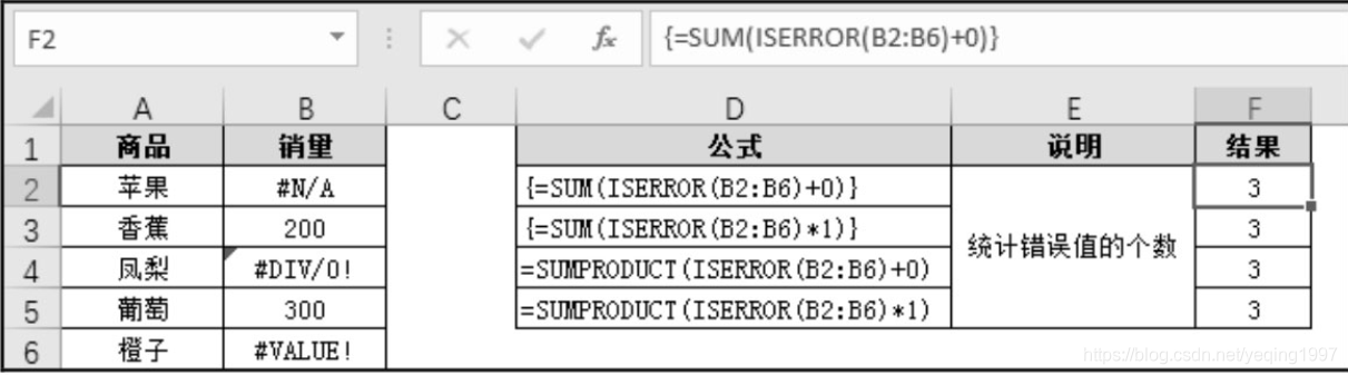
The iserror function
checks whether a value is an error (#N/A, #VALUE!, #REF!, #DIV/0!, #NUM!, #NAME?, #NULL!), and the result returns TRUE or FALSE.


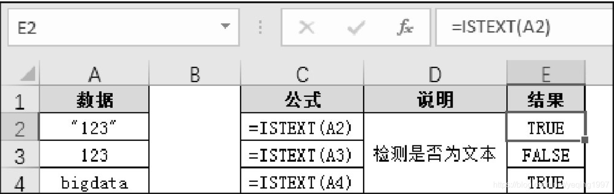
⑦istext function
checks whether a value is text, and returns TRUE or FALSE.

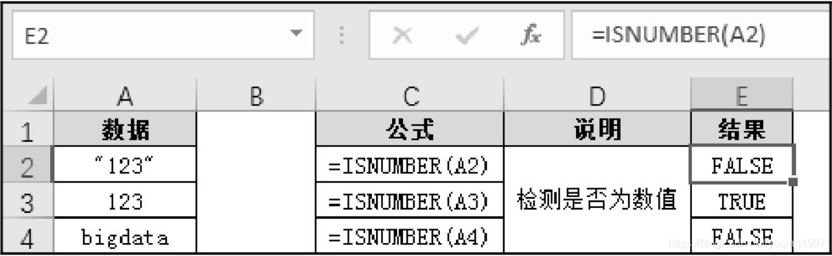
⑧isnumber function
checks whether a value is a number, and returns TRUE or FALSE.

5. The date calculation function
   gets the current date and time today and now functions, returns the year, month, and day functions of the date, hour, minute, and second functions that return the hour, minute, and second of the time, and splices the date The date function and the time function of splicing time, the weekday function for obtaining the day of the week and the weeknum function for calculating the week of the year, the calculation of the year, month, number of days, and the datedif, days, and networkdays functions of the weekday interval between two dates.
   ①today function
   
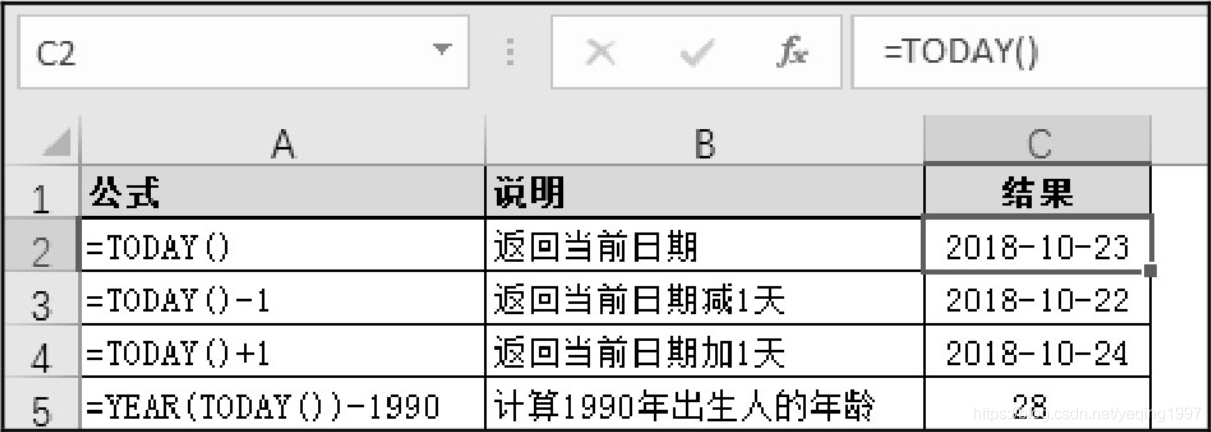
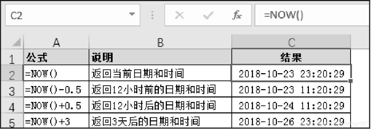
   ②now function
   Returns the serial number of the current date and time.
   
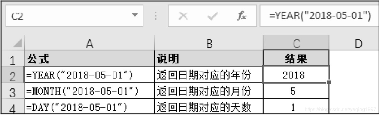
   ③The year, month, day function
   YEAR returns the year corresponding to a certain date, and YEAR is returned as an integer ranging from 1900 to 9999.
   MONTH returns the month in the date (represented as a serial number). The month is an integer between 1 and 12.
   DAY returns the number of days in a date expressed as a serial number. The number of days is an integer between 1 and 31.
   
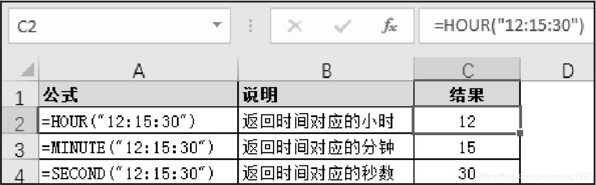
   ④hour, minute, second function
   HOUR returns the hour of the time value, hour is an integer ranging from 0 to 23;
   MINUTE returns the number of minutes of the time value, minute is an integer ranging from 0 to 59;
   SECOND returns the number of seconds of the time value , The number of seconds is an integer from 0 to 59.
   
   ⑤The
   date function returns a continuous serial number that represents a specific date.
   
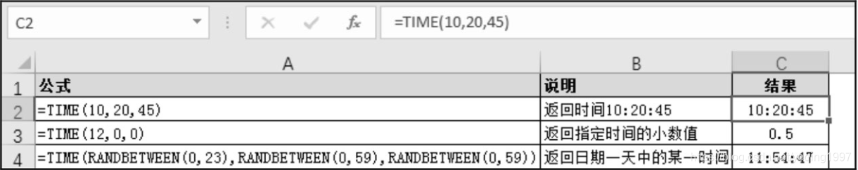
   ⑥time function
   Returns the decimal number of a specific time.
   
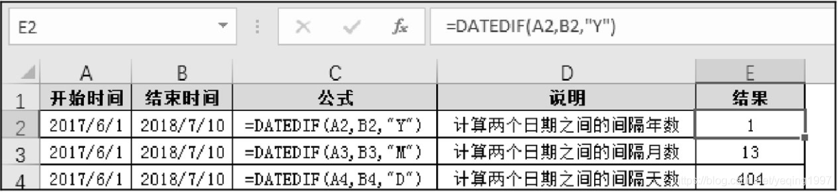
   ⑦Datedif function
   Calculate the number of years, months or days between two dates.
   

6. Matching search function To
   quickly find the value that matches a certain cell or range, you can use the matching search function in the Excel function, such as choose, vlookup, hlookup, lookup, match, index, offset, indirect, etc.
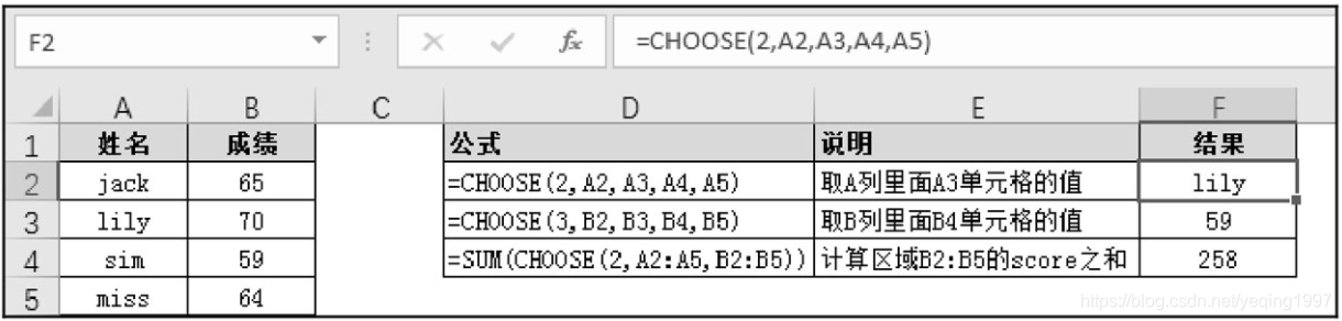
   ①The choose function
   returns the value in the numerical parameter list according to the index number index_num.
   
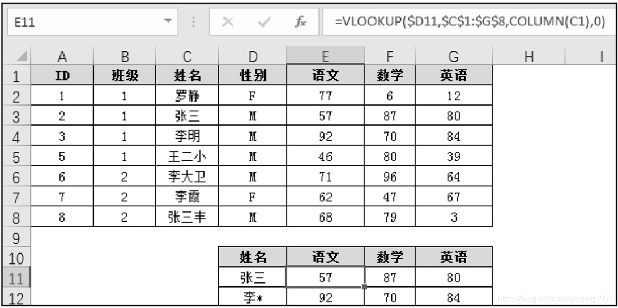
   ②The vlookup function
   searches the first column of the search value in a certain area, and returns the value of the col_index_num column on the right that is in the same line with the search value according to the column number.
   
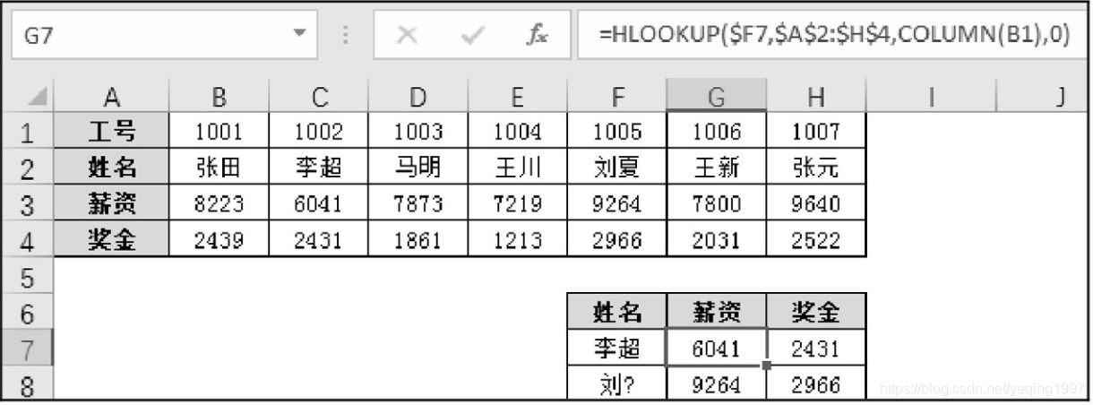
   ③The hlookup function
   searches the first row of the search value in a certain area, and returns the value of the row_index_num row below and the search value in the same column according to the row number.
   The functions of HLOOKUP and VLOOKUP are very similar, both are functions for matching search, and the function parameters are the same. The only difference is that the VLOOKUP function searches on the column, while the HLOOKUP function searches on the row.
   
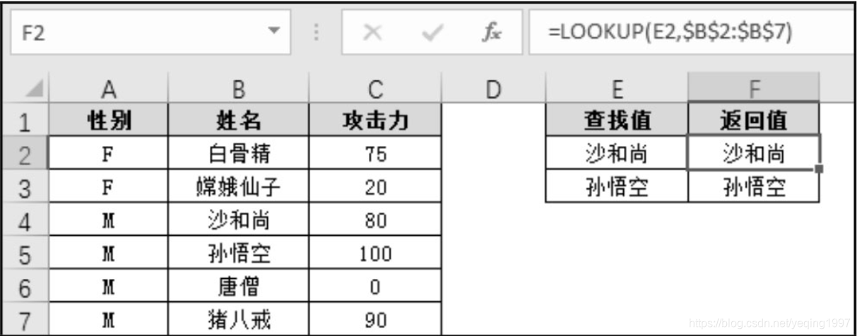
   ④The lookup function
   searches the lookup value in a row or column, and returns the value at the same position in the row or column. The LOOKUP function can perform exact matching and approximate matching.

Exact matching (the search range and the return range are the same)

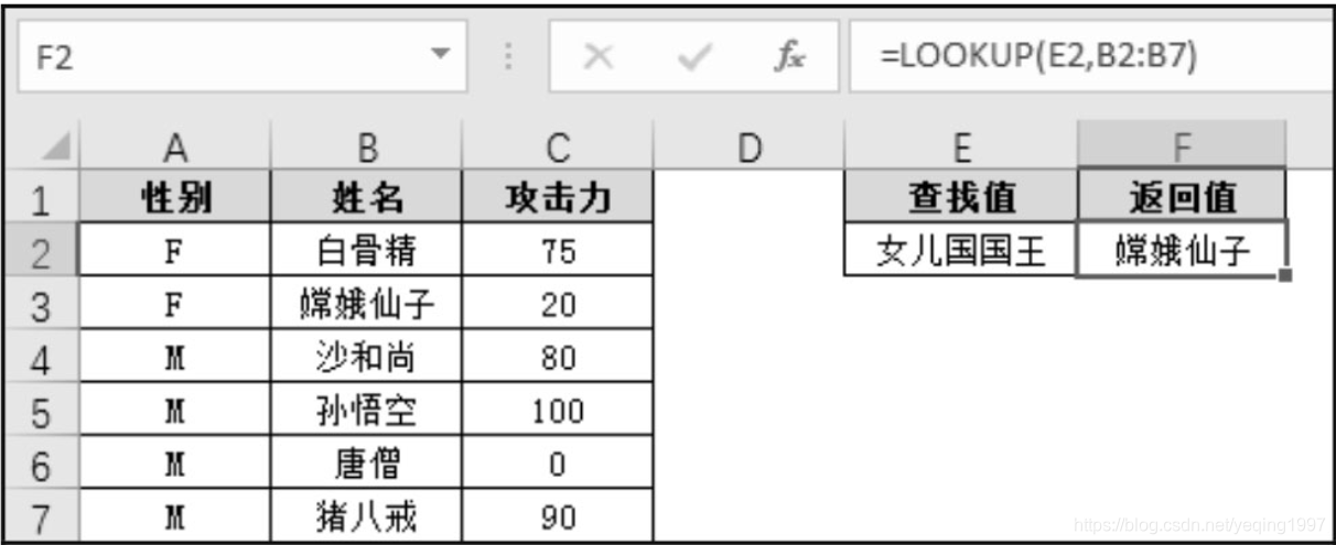
Approximate matching (the search range and the return range are the same) the

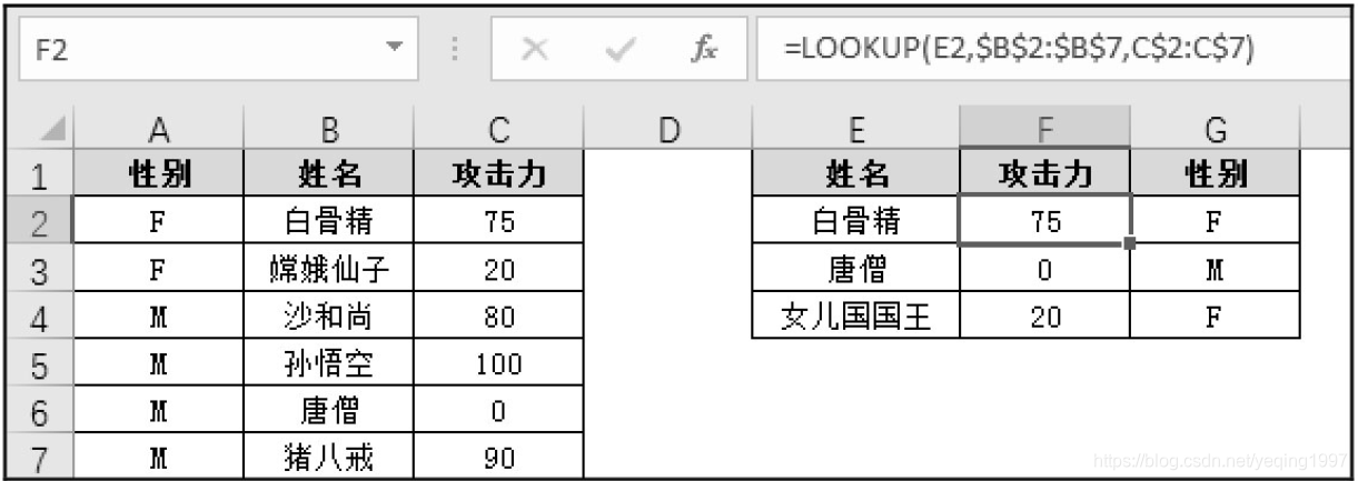
search range and the return range are inconsistent

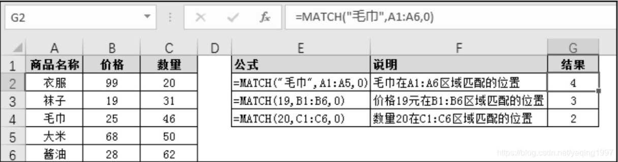
⑤match function
searches for a specific item in the area, and then returns the relative position of the item in this area.
Exact match

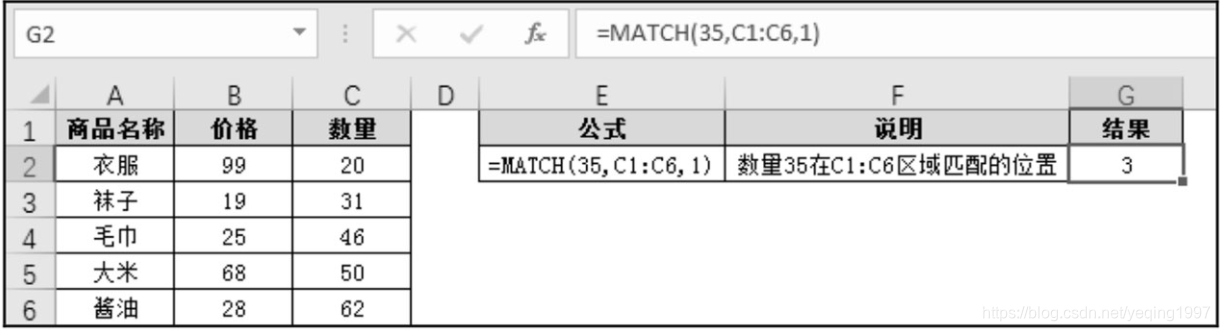
Approximate match

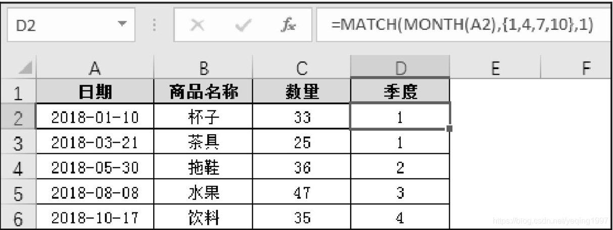
Judge the quarter according to the date. The

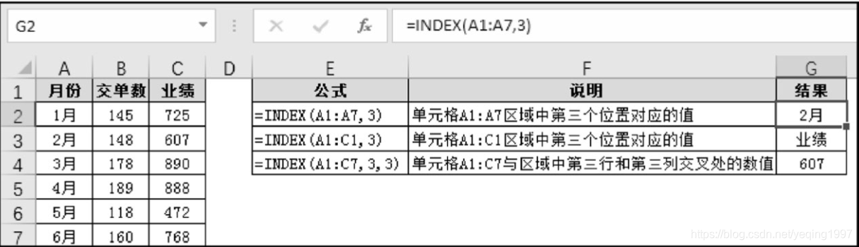
index function
returns the value or the reference of the value in the table or area.

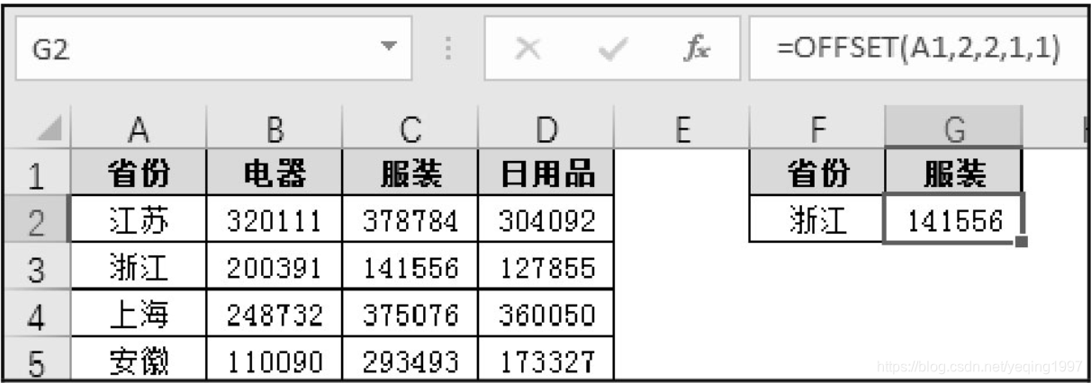
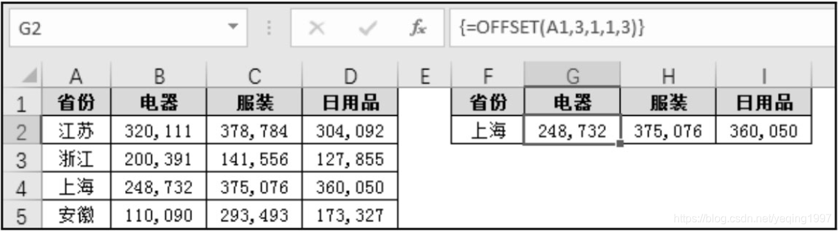
⑦The offset function
returns a reference to the range of the specified number of rows and columns in the cell or cell range. The reference returned can be a single cell or a range of cells.
Find and return the value of a certain cell

Find and return the value of the cell range

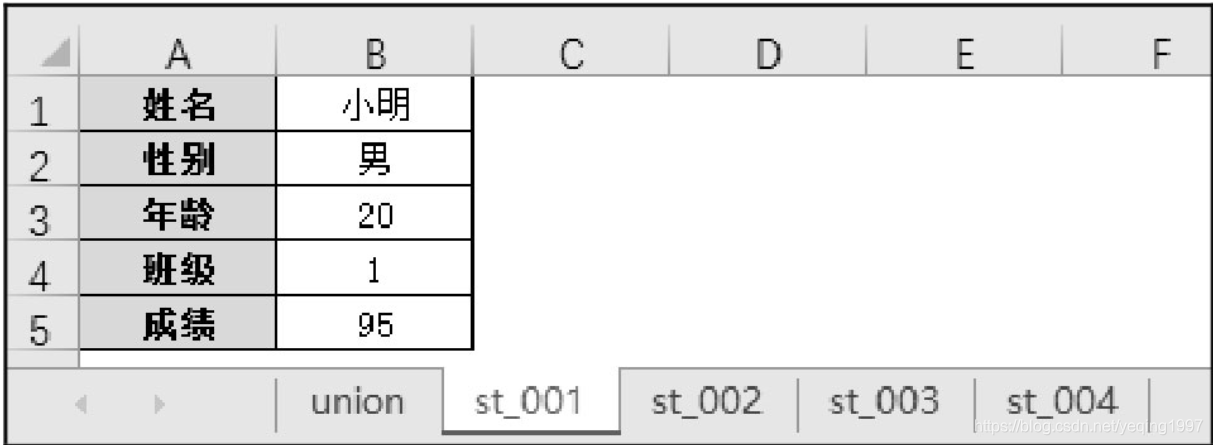
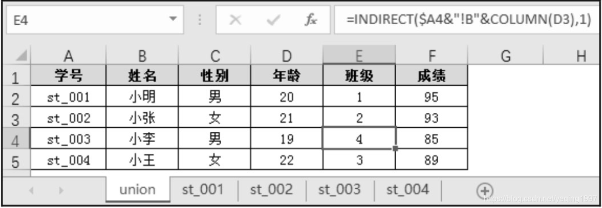
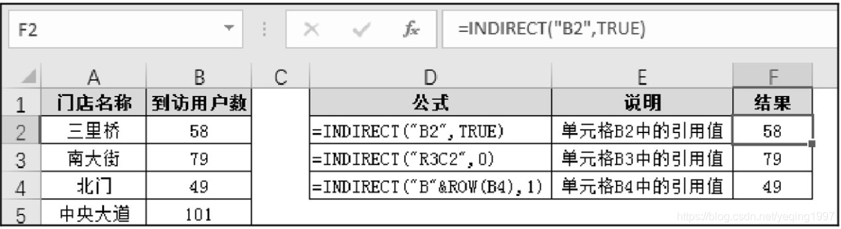
⑧indirect function
Returns the reference specified by the text string. This function immediately calculates the reference and displays its content.
Search returns the value of the specified cell

Multiple worksheets refer to merged data