Preliminary understanding of cellular automata
- Preliminary understanding of
cellular automata Cellular automata (CA) is a method used to simulate local rules and local connections. A typical
cellular automaton is defined on a grid. The grid at each point represents a cell and a finite
state. The change rule is applied to each cell and is performed simultaneously. - Cell Change Rule & Cell State
Typical change rule depends on the state of the cell and the state of its (4 or 8) neighbors. - Application of
Cellular Automata Cellular automata has been applied in the fields of physical simulation and biological simulation. - Matlab programming of cellular automata In
combination with the above, we can understand that cellular automata simulation needs to understand three points. One is a cell, which can be understood as a square block composed of one or more points in the matrix in matlab. Generally, we use a point in the matrix to represent a cell. The second is the change rule. The change rule of the cell determines the state of the cell at the next moment. The third is the state of the cell. The state of the cell is self-defined. It is usually an opposite state, such as the living state or death state of a creature, red or green light, obstacles or no obstacles at this point, etc. -
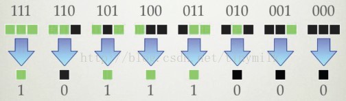
Here, we will discuss the application of the cell in the traffic flow model. As we all know, the simplest cellular traffic flow model is the 184th rule of elementary CA proposed by wolfram. Its evolution rules are as follows:
figure 1: Wolfram's rule 184
This rule allows the cell to simulate the feeling of traffic flow. Why is it a feeling, because everyone seems to see a square or a small car moving forward, but it does not simulate many phenomena in the traffic flow. Later, the NaSch rule was proposed. This rule can be said to be the originator of all cellular traffic flow models. Many of the following rules evolved from this rule. The two-lane model that we are discussing today for driving on the right is also improved based on the NaSch model. Let’s briefly discuss the NaSch model, and then further lead to the right driving model that this article will explain.
NaSch rules:
(1) Accelerate,
(2) Decelerate,
(3) Randomly slow down the speed with probability p,
(4) March,
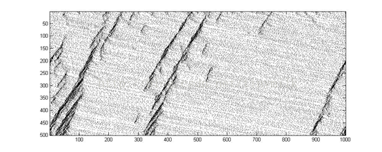
It can be seen that there are only four simple NaSch rules, but they simulate the most basic things of traffic flow, which can be seen from the time-space diagram:
figure 2:Density=0.15,Vmax=5
Figure 2 is the space-time diagram obtained when the cell length is 1000 and the time step is 500. There are corresponding basic maps including flow density map and velocity density map that can also be derived.
Next, we are one step closer to our right-driving model. Before that, we will introduce the two-lane model STNS based on NaSch. With the two-lane model, the right-driving model is no longer difficult.
STNS rules:
(1) Accelerate,
(2) Decelerate,
(3) Changing lanes meets the following conditions:
1. Motivation for changing lanes:
2. Safety conditions:
(4) Randomly slow down the speed with probability p,
(5) March,
It can be seen from the rules of STNS that in order to implement the two-lane CA traffic flow model, our actual change to the NaSch model is only to add a lane change rule, and the lane change rule seems to be so easy to understand and in line with realistic conditions. . This is the charm of CA. By slightly changing the rules, we can achieve some of the results we want. We will use the right-hand driving model to interpret this later. Of course, the rules are also a nightmare for CA. We usually don't know when to use what CA rules.
Now I will introduce another rule under which CA can realize the right driving rule in the 2014 MCM competition. At the same time, it can be expected that if some rules are modified, any of the problems in the 2014 MCM competition A can still be fully realized, but here This will not be discussed.
Keep-Right Rule:
1) Speed up,
(2) Decelerate,
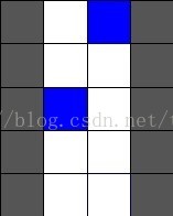
(3) The left lane meets the following conditions:
1. Motivation for changing lanes:
2. Safety conditions:
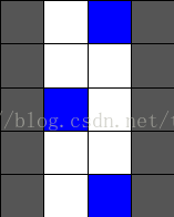
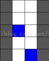
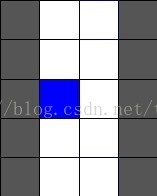
(4) Changing lanes to the right meets that the car can change lanes without a car within two squares on the right and the right side (this is also in accordance with the actual right-hand rule, if you can go back to the right lane and you will go back under the condition of ensuring safety) . The rules for image presentation are as follows:
figure 3
You can see that only the rightmost picture can change lanes to the right.
(5) Randomly slow down the speed with probability p,
(6) March,
At this point, the right-hand driving rule has been implemented using cellular automata. The following is a simulation diagram implemented with Matlab:
%%%%%%%%%%%%%%%%%%%%%%%%%%%%%%%%%%%%%%%%%%%%%%%%%%%%%%%%%%%%%%%%%%%%%%%%%%
% A Two-Lane Cellular Automaton Traffic Flow Model with the Keep-Right Rule
%%%%%%%%%%%%%%%%%%%%%%%%%%%%%%%%%%%%%%%%%%%%%%%%%%%%%%%%%%%%%%%%%%%%%%%%%%
clc;
clear all;
close all;

B=3;              % The number of the lanes
plazalength=100;  % The length of the simulation highways
h=NaN;            % The handle of the image


[plaza,v]=create_plaza(B,plazalength);
h=show_plaza(plaza,h,0.1);

iterations=1000;    % Number of iterations
probc=0.1;          % Density of the cars
probv=[0.1 1];      % Density of two kinds of cars
probslow=0.3;       % The probability of random slow
Dsafe=1;            % The safe gap distance for the car to change the lane
VTypes=[1,2];       % Maximum speed of two different cars
[plaza,v,vmax]=new_cars(plaza,v,probc,probv,VTypes);% Generate cars on the lane

size(find(plaza==1))
PLAZA=rot90(plaza,2);
h=show_plaza(PLAZA,h,0.1);
for t=1:iterations;
    size(find(plaza==1))
    PLAZA=rot90(plaza,2);
    h=show_plaza(PLAZA,h,0.1);
    [v,gap,LUP,LDOWN]=para_count(plaza,v,vmax);
    [plaza,v,vmax]=switch_lane(plaza,v,vmax,gap,LUP,LDOWN);
    [plaza,v,vmax]=random_slow(plaza,v,vmax,probslow);
    [plaza,v,vmax]=move_forward(plaza,v,vmax);
end

Complete code or write on behalf of adding QQ1575304183