1. Introduction
1. Cells
Cells can also be called units. Or primitive, is the most basic part of cellular automata. The cells are distributed on discrete one-dimensional, two-dimensional or multi-dimensional Euclidean lattice points.
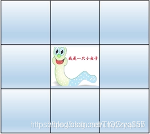
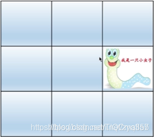
Each cell has a state, for example, the state of the cell in the middle below is a small bug, and the other cells are in a state without small bugs. But if the bug moves, it is the result of the change of state over time
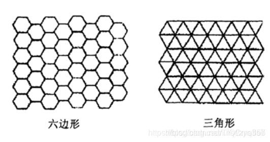
There are many kinds of cells, which can be hexagons, triangles, etc. We can deal with specific problems specifically.
2. Cell space The
set of spatial mesh points where the cells are distributed is the cell space here.
3. Neighbors
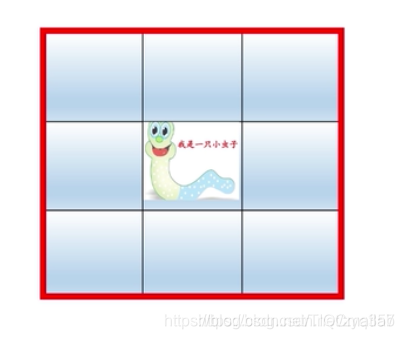
In a one-dimensional cellular automaton, the radius is usually used to determine the neighbors. A distance from a cell, all cells within are considered to be neighbors of the cell. The neighbor definition of a two-dimensional cellular automaton is more complicated, but usually has the following forms (we take the most commonly used regular tetragonal grid division as an example). In the figure below, the black cell is the central cell, and the gray cell is its neighbor. Their states are used to calculate the state of the central cell at the next moment.
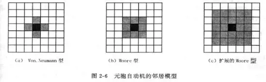
In other words: the state of a cell at the next moment is determined by its own state and the state of its neighbor cells.
4. Rules
Rules are one of the most important points, which determine the quality of the cellular algorithm.
Cellular automata is the interaction between local cells according to rules to cause global changes.
Second, the source code
% DLA
clc;clear;close all;
S=zeros(400,500); % 生成状态矩阵
S(end,:)=1; % 设置状态矩阵中最下面一行元素等于1
A=1;B=1;X=0.8;
rand('state',0); % 设置随机数的状态数
subplot(121);Ii=imshow(1-S,[]); % 显示状态矩阵
T1=title(['times = 1',', total particle=',num2str(sum(S(:)))],...
    'Fontname','times new roman','fontsize',14); % 显示时间与粒子总数
r=rand(1,500);
subplot(122);P1=plot(sum(S,2)/size(S,2),1:size(S,1),'r');% 绘制各行的密度值曲线
set(gca,'Position',[0.57,0.35,0.33,0.36],'YDir','reverse'); % 设置坐标轴属性
xlim([0,max(sum(S,2)/size(S,2))]); % 设置x轴的范围
ylabel('\ith','fontname','times new roman','fontsize',14); % y轴标注
xlabel('\it\rho','fontname','times new roman','fontsize',14); % x轴标注
title('{\it\rho} ({\ith})','fontname','times new roman','fontsize',14); % 加注图题
set(gcf,'DoubleBuffer','on'); % 设置图形窗口的渲染效果
[L1,L2]=size(S); % 返回状态矩阵的行数L1和列数L2
N=500;H=1; % 初始化参数:粒子总数N和时间参数H
h=150; % 设置截顶高度
scale=0.5; % 设置剪切系数
while N<20000;
    R1=2+round([L1-3]*rand); % 随机产生粒子的坐标
    R2=2+round([L2-4]*rand); % 随机产生粒子的坐标
    flag=0; % 控制循环停止的参数
    while R1<L1&R1>1&R2<L2&R2>1&flag==0; % 验证粒子在状态矩阵内部且粒子未被吸附
        he=S(R1,R2-1)+S(R1,R2+1)+S(R1+1,R2); % 计算左、下和右方位的近邻
        if he>0.5; % 判断近邻中有固定粒子
            S(R1,R2)=1; % 运动粒子被吸附
            flag=1; % 标记粒子已经被吸附
        else
            ra=rand; % 粒子进行随机移动的分量
            rb=rand; % 粒子进行随机移动的分量
            R1=R1+(ra>=0.5)-(ra<0.5); % 计算下一时刻粒子的位置坐标
            R2=R2+(rb>=0.5)-(rb<0.5); % 计算下一时刻粒子的位置坐标
        end
    end
    sS=sum(S,2); % 对行所有元素求和
    Se=find(sS);Se=min(Se); % 找出有粒子的最高一行
    if Se==[size(S,1)-h]; % 判断高度是否达到截顶高度
        Sx=find(S(Se,:)); % 找出最高点粒子的横坐标
        S=cuth(S,h,Se,Sx,scale); % 切去最高点粒子所在的分支
    end
    set(Ii,'CData',1-S); % 显示状态矩阵
    N=sum(S(:)); % 计算粒子总数
    H=H+1; % 累计时间值
    set(P1,'XData',sum(S,2)/size(S,2)); % 更新密度曲线数据
    set(T1,'string',['times = ',num2str(H),', total particle=',num2str(sum(S(:)))]);% 更新时间和粒子总数
    pause(0.02); % 暂停一下,显示动画效果
end
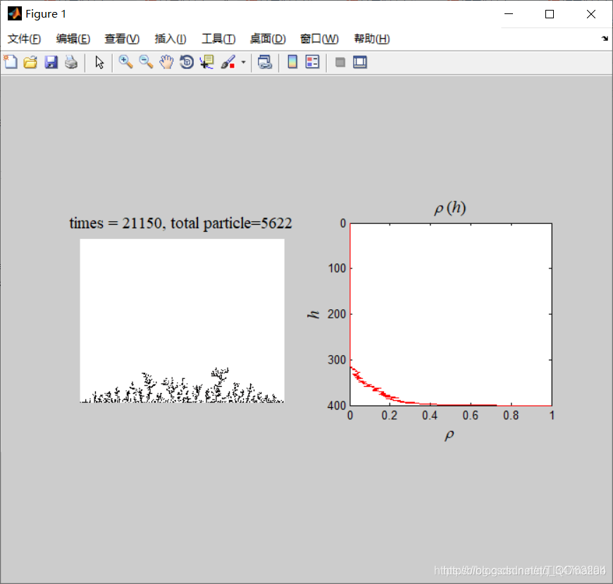
Three, running results
Four, remarks
Complete code or writing to add QQ2449341593 past review
>>>>>>
[Cellular Automata] Two-lane traffic flow model based on Matlab cellular automata, including right-hand driving [including Matlab source code 231]