Python simulates common distributions and does related hypothesis tests

1. Common distribution

According to whether the random variable type is discrete or continuous (the number of values ​​is finite or infinite), the event distribution can be divided into discrete distribution and continuous distribution.

Common discrete distributions are:

• Binomial distribution (Bernoulli distribution)
• Poisson distribution
• Geometric distribution
• Negative binomial distribution
• Hypergeometric distribution

Common continuous distribution:

• Evenly distributed
• index distribution
• Normal distribution

1.1 Generate random variables with a specific distribution

Python generates random distribution mainly using Numpy and Scipy's stats, the code is as follows:

• Discrete random variable

import numpy as np
s=np.random

#二项分布，参数为试验次数与每次成功概率
s.binomial(10,0.6,10)
array([8, 4, 4, 7, 4, 5, 5, 7, 7, 6])

#二项分布，参数为试验次数与每次成功概率
s.binomial(10,0.6,10)
array([8, 4, 4, 7, 4, 5, 5, 7, 7, 6])

#几何分布，参数为成功概率
s.geometric(0.6,(10,))
array([1, 1, 1, 2, 3, 1, 2, 1, 1, 1])

#返回成功3次，每次成功概率为0.6，前会失败的次数
s.negative_binomial(3,0.6,10)
array([1, 1, 2, 0, 1, 6, 4, 0, 3, 1])

#参数为关注事物的数量，不关注事物的数量，采样的数量，实验次数
#返回为样本中包含关注事物的个数
s.hypergeometric(10,5,2,10)
array([1, 0, 1, 2, 2, 0, 1, 2, 2, 2])

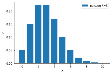
As λ becomes larger and larger, the Poisson distribution becomes more symmetrical and closer to the normal distribution.

• Continuous random variable

#正态分布，均值，标准差，试验次数
s.normal(0,1,10)
s.standard_normal(10)
array([-1.3756928 , -0.69395138, -0.05536103, -0.49320461,  0.53539012,
       -0.65562987, -0.60314098,  0.53543226,  0.23511523,  0.1169497 ])

#指数分布,单位时间接待3个客户，那么下一个客户需要的时间为多少，这里试验10次。注意该方法参数为指数分布参数λ的倒数
s.exponential(1/3,10)
array([0.04577549, 0.04436587, 0.0040138 , 0.0359573 , 0.65450092,
       0.58551778, 0.02194068, 0.01608489, 0.01789454, 0.04151969])

1.2 Calculate the distribution function of the statistical distribution

Use probability to describe the distribution of variables. For discrete random variables, the probability mass function (PMF) is used to describe its distribution. For continuous random variables, use probability density function (PDF) and cumulative function to describe its distribution.

l=range(10)
#二项分布的概率
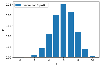
stats.binom.pmf(l,10,0.6)

#array([1.04857600e-04, 1.57286400e-03, 1.06168320e-02, 4.24673280e-02,
#       1.11476736e-01, 2.00658125e-01, 2.50822656e-01, 2.14990848e-01,
#       1.20932352e-01, 4.03107840e-02])

#泊松分布概率
stats.poisson.pmf(l,mu=3)

#array([0.04978707, 0.14936121, 0.22404181, 0.22404181, 0.16803136,
#      0.10081881, 0.05040941, 0.02160403, 0.00810151, 0.0027005 ])

Binomial distribution probability mass function:

Poisson distribution probability mass function:

# 计算均匀分布U(0,1)的PDF
x = np.linspace(1,3,10)
#loc起始位置，scale区间长度
stats.uniform.pdf(x,loc=1, scale=2)
#array([0.5, 0.5, 0.5, 0.5, 0.5, 0.5, 0.5, 0.5, 0.5, 0.5])

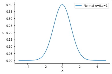
# 计算正态分布N(0,1)的PDF
x = np.linspace(-3,3,10)
stats.norm.pdf(x,loc=0, scale=1)

#array([0.00443185, 0.02622189, 0.09947714, 0.24197072, 0.37738323,
#       0.37738323, 0.24197072, 0.09947714, 0.02622189, 0.00443185])

# 计算指数分布E(1)的PDF
x = np.linspace(0,10,10)
#scale为指数分布参数λ
stats.expon.pdf(x,loc=0,scale=1)

#array([1.00000000e+00, 3.29192988e-01, 1.08368023e-01, 3.56739933e-02,
#       1.17436285e-02, 3.86592014e-03, 1.27263380e-03, 4.18942123e-04,
#       1.37912809e-04, 4.53999298e-05])

Normal distribution probability density function:

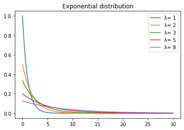
exponential function probability density function:

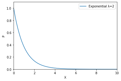
as λ becomes larger, the waiting time changes:

2. Hypothesis testing

The stats module of scipy can also do hypothesis testing conveniently

2.1 Normal hypothesis test

Shapiro-Wilk test to do normal hypothesis test

from scipy.stats import shapiro
data_nonnormal = np.random.exponential(size=100)
data_normal = np.random.normal(size=100)

def normal_judge(data):
    stat, p = shapiro(data)
    if p > 0.05:
        return 'stat={:.3f}, p = {:.3f}, probably gaussian'.format(stat,p)
    else:
        return 'stat={:.3f}, p = {:.3f}, probably not gaussian'.format(stat,p)

# output
normal_judge(data_nonnormal)
'stat=0.827, p = 0.000, probably not gaussian'

2.2 Independence test (chi-square test)

• Chi-square test
  Purpose: To test whether the two groups of categorical variables are related or independent

  H0: The two samples are independent

  H1: The two sets of samples are not independent

from scipy.stats import chi2_contingency
table = [[10, 20, 30],[6,  9,  17]]
#stat统计量，p显著度，dof自由度，expected期望边界
stat, p, dof, expected = chi2_contingency(table)
print('stat=%.3f, p=%.3f' % (stat, p))
if p > 0.05:
	print('Probably independent')
else:
	print('Probably dependent')
	
stat=0.272, p=0.873
Probably independent

expected
array([[10.43478261, 18.91304348, 30.65217391],
       [ 5.56521739, 10.08695652, 16.34782609]])

2.3 Mean test

• T-test
  purpose: to test whether the means of two independent sample sets are significantly different (and then determine whether the distributions are the same, because the variances are the same by default)

  H0: Means are equal

  H1: Means are not equal

from scipy.stats import ttest_ind
data1 = np.random.normal(size=10)
data2 = np.random.normal(size=10)
#这里默认总体方差相同，判断两者均值是否相同
stat, p = ttest_ind(data1, data2)
print('stat=%.3f, p=%.3f' % (stat, p))
if p > 0.05:
	print('Probably the same mean value')
else:
	print('Probably different mean value')

stat=-0.761, p=0.457
Probably the same mean value

• ANOVA
  purpose: similar to t-test, ANOVA can test whether the means of two or more independent sample sets are significantly different

  H0: Means are equal

  H1: Means are not equal

from scipy.stats import f_oneway
data1 = np.random.normal(size=10)
data2 = np.random.normal(size=10)
data3 = np.random.normal(size=10)
stat, p = f_oneway(data1, data2, data3)
print('stat=%.3f, p=%.3f' % (stat, p))
if p > 0.05:
	print('Probably the same distribution')
else:
	print('Probably different distributions')
 
# output
# stat=0.189, p=0.829
# Probably the same distribution

2.4 Identical distribution test

• Mann-Whitney U Test
  Purpose: To test whether the distributions of two sample sets are the same (to directly judge whether the distributions are consistent)

  H0: The distribution of the two sample sets is the same

  H1: The distribution of the two sample sets is different

from scipy.stats import mannwhitneyu
data1 = [0.873, 2.817, 0.121, -0.945, -0.055, -1.436, 0.360, -1.478, -1.637, -1.869]
data2 = [1.142, -0.432, -0.938, -0.729, -0.846, -0.157, 0.500, 1.183, -1.075, -0.169]
stat, p = mannwhitneyu(data1, data2)
print('stat=%.3f, p=%.3f' % (stat, p))
if p > 0.05:
	print('Probably the same distribution')
else:
	print('Probably different distributions')

# output
# stat=40.000, p=0.236
# Probably the same distribution

reference

This content comes from the DataWhale probability statistics team study.