Dimension reduction and visualization of iris flower dataset with PCA

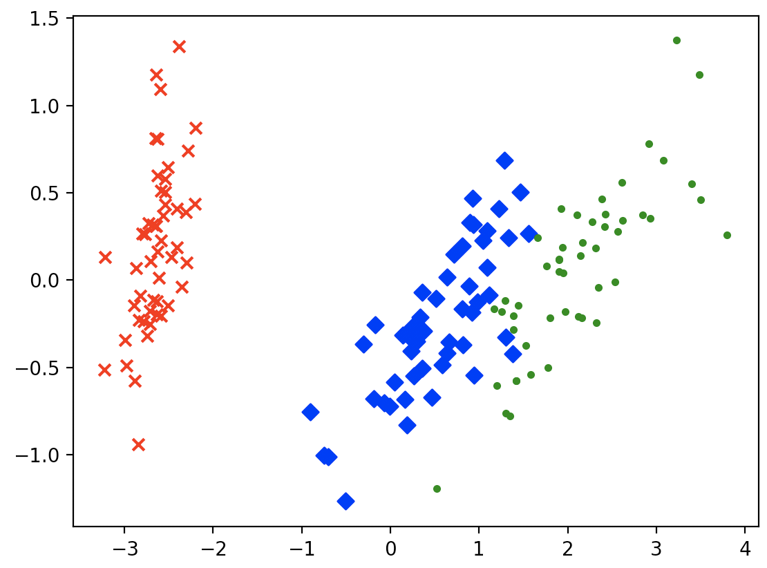
In the last blog , we introduced and implemented the PCA algorithm using code. In this blog, we applied the PCA algorithm to reduce the dimensionality and visualize the iris dataset.

Introduction to the iris dataset

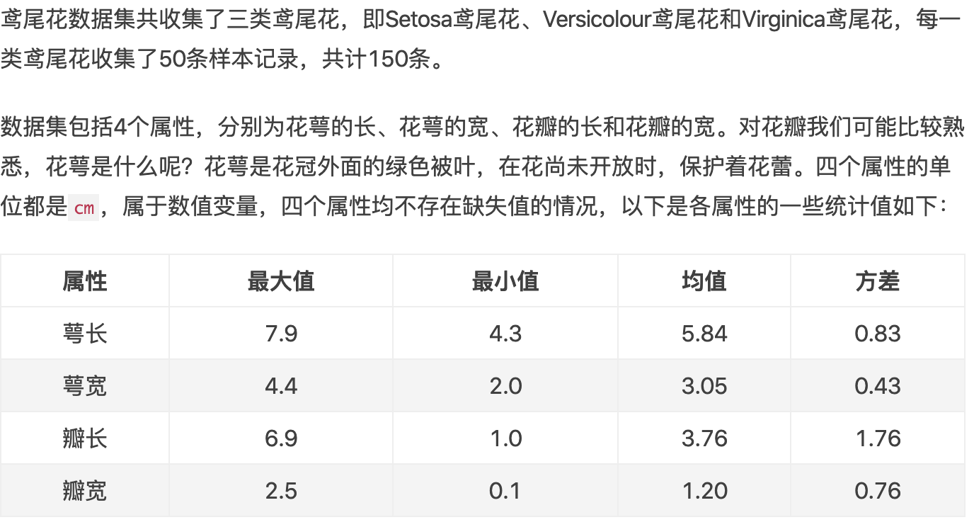
Code

The following code is from the "Python Machine Learning Application" course on MOOC .

import matplotlib.pyplot as plt 
from sklearn.decomposition import PCA 
from sklearn.datasets import load_iris 

data = load_iris () # load the iris data set in dictionary form 
y = data.target # use y to represent the label in the data set 
X = data.data # Use X to represent the attribute data in the data set 
pca = PCA (n_components = 2) # Load the PCA algorithm and set the number of principal components after dimensionality reduction to 2 
reduced_X = pca.fit_transform (X) # Reduce the dimensionality of the original data and save it in reduced_X Medium 

red_x, red_y = [], [] # first type data point 
blue_x, blue_y = [], [] # second type data point 
green_x, green_y = [], [] # third type data point 

for i in range (len (reduced_X)): # Save the dimensionality-reduced data points in different lists according to the iris category. 
    if y [i] == 0:  
        red_x.append (reduced_X [i] [0])
        red_y.append (reduced_X [i] [1]) 
    elif y [i] == 1:
        blue_x.append(reduced_X[i][0])
        blue_y.append(reduced_X[i][1])
    else:
        green_x.append(reduced_X[i][0])
        green_y.append(reduced_X[i][1])

plt.scatter(red_x, red_y, c='r', marker='x')
plt.scatter(blue_x, blue_y, c='b', marker='D')
plt.scatter(green_x, green_y, c='g', marker='.')
plt.show()

operation result:

 

References

[1] Iris data set