[Sklearn] dimensionality reduction processing PCA&SVD

One, the dimensionality reduction algorithm in sklearn

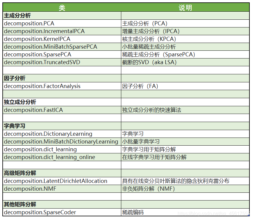
The dimensionality reduction algorithms in sklearn are all included in the module decomposition, which is essentially a matrix decomposition module. In the past ten years, if you want to discuss the pioneer of algorithm progress, matrix decomposition can be said to be unique. Matrix decomposition can be used in dimensionality reduction, deep learning, cluster analysis, data preprocessing, low-latitude feature learning, recommendation systems, big data analysis and other fields.

2. PCA and SVD

There are a variety of important feature selection methods in feature engineering: variance filtering. If the variance of a feature is small, it means that a large number of values ​​of this feature are likely to be the same (for example, 90% are 1, only 10% are 0, or even 100% are 1), then the value of this feature For the sample, there is no discrimination, and this feature does not carry valid information. From this application of variance, it can be inferred that if a feature has a large variance, it means that the feature contains a lot of information .
Therefore, in dimensionality reduction,The information measurement indicator used by PCA is the sample variance, also known as interpretable variance. The larger the variance, the more information the feature carries.

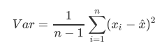
Var represents the variance of a feature, n represents the sample size, xi represents the value of each sample in a feature, and xhat represents the mean of this list of samples.

2.1 Realization of dimensionality reduction

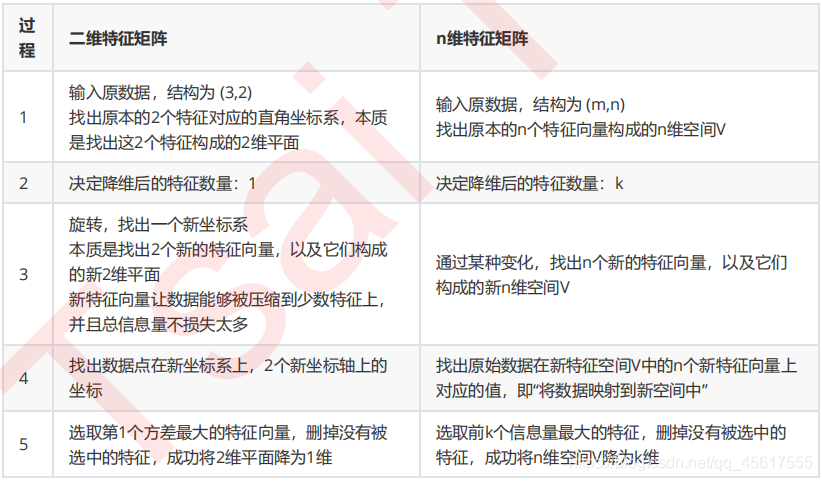
In step 3, the technique we use to find n new feature vectors so that the data can be compressed to a few features without losing too much total information ismatrix decomposition. PCA and SVD are two different dimensionality reduction algorithms, but they both follow the above process to achieve dimensionality reduction, but the method of matrix decomposition in the two algorithms is different, and the measurement index of the amount of information is different.

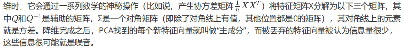
1. PCA

PCA uses variance as a measure of the amount of information, and eigenvalue decomposition to find the space V.

2.SVD

3. The difference between PCA and feature selection technology

• PCA is to compress the existing features, and the features after dimensionality reduction are not any one of the original feature matrix, but a combination of features.
• Feature selection technology: select the most information-carrying feature from the existing features, and the features after the selection are still interpretable.
  Therefore: you can imagine,PCAgeneralNot applicableinExplore the relationship between features and labelsModel (such as linear regression) because the relationship between the unexplainable new feature and the label is not meaningful. In linear regression models, we use feature selection.

Three, sklearn code implementation

3.1 PCA performs dimensionality reduction visualization on the iris data set

import matplotlib.pyplot as plt
from sklearn.datasets import load_iris
from sklearn.decomposition import PCA

iris = load_iris()
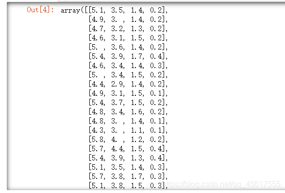
X=iris.data
y=iris.target
X.shape

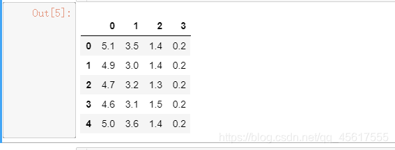
import pandas as pd
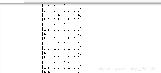
pd.DataFrame(X).head()

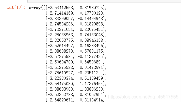
# 使用PCA降到两维
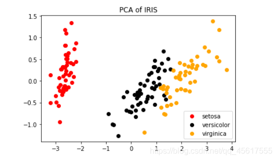
tr_X = PCA(2).fit_transform(X)
tr_X

color=['red','black','orange']
iris

plt.figure()
for i in [0,1,2]:
    plt.scatter(tr_X[y==i, 0]
               , tr_X[y==i, 1]
               , c=color[i]
               , label=iris.target_names[i])
plt.legend()
plt.title('PCA of IRIS')
plt.show()

#属性explained_variance_，查看降维后每个新特征向量上所带的信息量大小（可解释性方差的大小）
pca.explained_variance_#查看方差是否从大到小排列，第一个最大，依次减小

#属性explained_variance_ratio，查看降维后每个新特征向量所占的信息量占原始数据总信息量的百分比
#又叫做可解释方差贡献率
pca.explained_variance_ratio_

import numpy as np
pca_line = PCA().fit(X)
# pca_line.explained_variance_ratio_#array([0.92461872, 0.05306648, 0.01710261, 0.00521218])
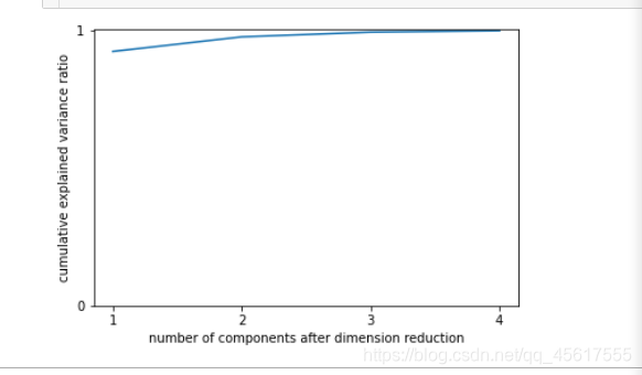
plt.plot([1,2,3,4],np.cumsum(pca_line.explained_variance_ratio_))
plt.xticks([1,2,3,4]) #这是为了限制坐标轴显示为整数
plt.yticks([0,1])
plt.xlabel("number of components after dimension reduction")
plt.ylabel("cumulative explained variance ratio")
plt.show()

3.2 PCA uses random forest algorithm to find optimal parameters after dimensionality reduction

from sklearn.decomposition import PCA
from sklearn.ensemble import RandomForestClassifier as RFC
from sklearn.model_selection import cross_val_score
import matplotlib.pyplot as plt
import pandas as pd
import numpy as np

data = pd.read_csv(r".\digit recognizor.csv")
X=data.iloc[:,1:]
y=data.iloc[:,0]

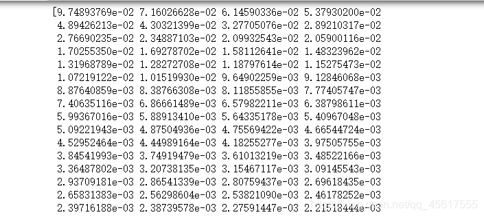
pca_line=PCA().fit(X)
print(pca_line.explained_variance_ratio_)

Data after dimensionality reduction:

plt.figure()
plt.plot(np.cumsum(pca_line.explained_variance_ratio_))
plt.xlabel("number of components after dimension reduction")
plt.ylabel("cumulative explained variance ratio")
plt.show()

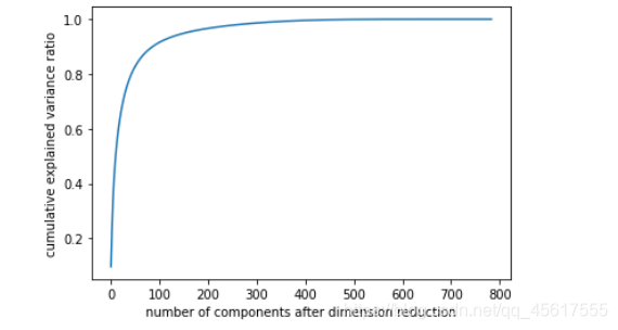
Judging that it is best to reduce to a few-dimensional model

score=[]
for i in range(1,101,10):
    tr_X=PCA(i).fit_transform(X)
    once = cross_val_score(RFC(n_estimators=10,random_state=0)
                           ,tr_X,y,cv=5).mean()
    score.append(once)
plt.figure(figsize=[20,5])
plt.plot(range(1,101,10),score)
plt.show()

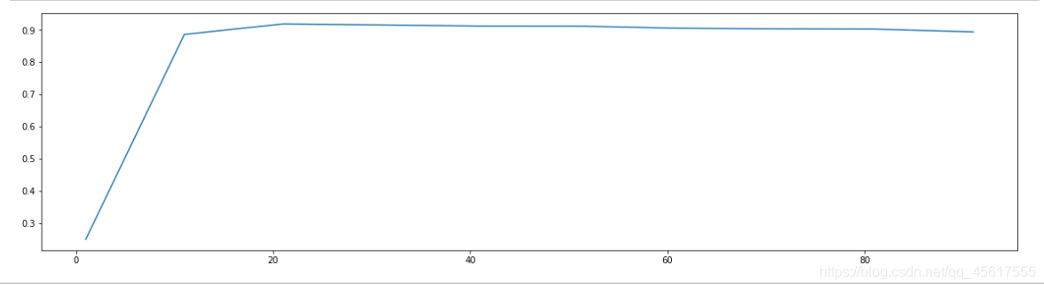
Found between 10-25:
cross-validation method!

score = []
for i in range(10,25):
    X_dr = PCA(i).fit_transform(X)
    once = cross_val_score(RFC(n_estimators=10,random_state=0),X_dr,y,cv=5).mean()
    score.append(once)
plt.figure(figsize=[20,5])
plt.plot(range(10,25),score)
plt.show()

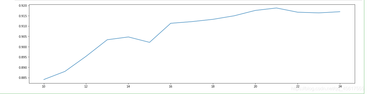
Found that dimensionality reduction to 25 is the best

X_dr = PCA(22).fit_transform(X)
 
#======【TIME WARNING:1mins 30s】======#
cross_val_score(RFC(n_estimators=100,random_state=0),X_dr,y,cv=5).mean()#0.946524472295366

3.3 Use KNN to find optimal parameters after PCA dimensionality reduction

The usage of cross-validation!

#======【TIME WARNING: 】======#

score = []
for i in range(10):
    X_dr = PCA(22).fit_transform(X)
    once = cross_val_score(KNN(i+1),X_dr,y,cv=5).mean()
    score.append(once)
plt.figure(figsize=[20,5])
plt.plot(range(10),score)
plt.show()

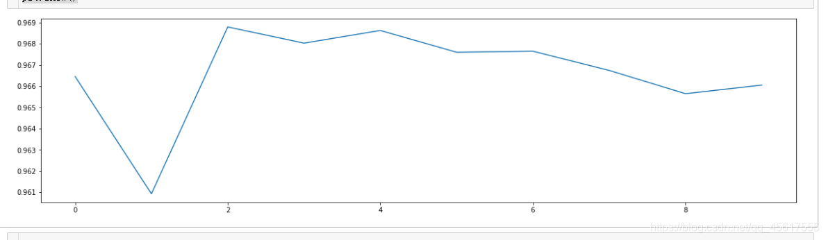
The optimal parameter is 2